In general machine learning applications performance evaluation is based on accuracy metrics, that are based on correct versus incorrect ratio.

In biometrics is more important to consider the rate of errors than the rate of correct answers.

Counting errors is not enough to evaluate the system, there is also the need to compute the rate between the errors and not-error. We will in fact consider measures like False Rejection Rate and the most critical for security False Acceptance Rate.

Threshold (in Biometric Verification)

In verification, the subject that presents the probe and the claim is accepted only if the similarity between the probe and the template in the gallery is higher than a certain set threshold. (The opposite if we’re using distances).

In identification, the threshold separates the “good templates” from the “bad templates”.

In general, a threshold is a value between 0 and 1 that tells when a certain similarity is enough.

A good threshold can only be chosen after a good performance evaluation, in which a different value for the threshold is chosen every iteration in order to see how the system behaves.

Of course, a threshold of 0 and 1 is not useful since a similarity of 1 (or a distance of 0) is impossible in real scenarios.

Biometric identification needs some flexibility. During the choosing of the acceptance threshold, there are also some downsides, so the designer has to find a balanced compromise. Remember that the most important value to consider is the error rate.

False Acceptance Rate and False Rejection Rate

Before defining what false acceptans rate and false rejection rate are, let’s introduce some notation:

$i d (p_{i})$ : returns the real identity of the probe $p_{i}$ or the template $g_{x}$ in the gallery.
$t o pM a t c h (p_{j}, i d e n t i t y)$ : returns the best match between $p_{j}$ and the possibly more than one templates associated to the claimed identity in the gallery.
$s (t_{1}, t_{2})$ : returns the similarity between two templates.

False Acceptance Rate (FAR): defines how many impostors access the system, out of all the impostors attempts to access the system. It’s better defined as $\frac{Num of probes with non genuine identity and similarity above t}{Number of non genuine attempts}$ :

F A R (t) = \frac{∣ { p _{j} : s _{x j} \geq t \land i d ( g _{x} ) \neq = i d ( p _{j} )} ∣}{∣ { p _{j} : i d ( g _{x} ) \neq = i d ( p _{j} )} ∣}

False Rejection Rate (FRR): defines how many genuine users cannot access the system because they’re rejected, out of all the genuine users attempts to access the systems. It’s better defined as $\frac{Num of probes with genuine identity and similarity below t}{Number of genuine attempts}$

FRR (t) = \frac{∣ { p _{j} : s _{x j} \leq t \land i d ( g _{x} ) = i d ( p _{j} )} ∣}{∣ { p _{j} : i d ( g _{x} ) = i d ( p _{j} )} ∣}

If we want to use Machine Learning terms, we can define $FRR = \frac{FN}{TP + FN}$ and $F A R = \frac{FP}{FP + TN}$ . We can see how they’re very different from other ML performance evaluation measures such precision an recall, since these last two are based on correct results, and FRR and FAR are based on errors (that’s the thing to minimize more in biometric systems).

N.B. Impostors can come from $P_{G} \cap P_{N}$ but genuine users can only come from $P_{G}$ .

Genuine Acceptance Rate and Genuine Rejection Rate

We define $T I$ as the True Impostor attempts, $TG$ as the True Genuine attempts. This values depends on the type of recognition (identification or verification).

The Genuine Acceptance Rate (GAR) is the number of genuine acceptances over the number of all the genuine claims.

G A R = \frac{G A}{TG}

On the other hand, the Genuine Rejection Rate (GRR) ****is the number of genuine rejections, over the number of all impostor claims.

GRR = \frac{GR}{T I}

Note that $FRR + G A R = 1$ and $F A R + GRR = 1$ .

Impostor and Client score distributions

In order to define these distributions, we have to define the two hypothesis:

$H_{0}$ : the person is a different person as the claimed identity;
$H_{1}$ : the person is the same person as the claimed identity.

The impostor distribution describes the probability of a similar value $s$ given that the hypothesis $H_{0}$ is true.

The impostor distribution is the same as the FAR distribution, and it’s given by the probability of having a decision $D_{1}$ in the presence of an hypothesis $H_{0}$ that’s true.

F A R = P (D_{1} ∣ H_{0})

On the other hand, the client score distribution (genuine distribution) is described as the FRR distribution, given by the probability of having a decision $D_{0}$ in the presence of an hypothesis $H_{1}$ that’s true.

FRR = P (D_{0} ∣ H_{1})

Both the distributions are normal distributions, meaning that most of the genuine and impostor acceptance will concentrate on two different values.

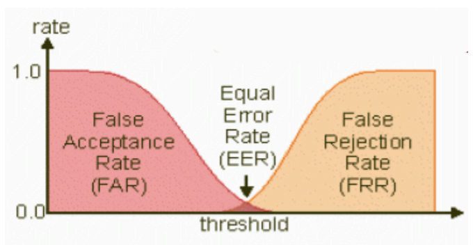
Equal Error Rate

FAR and FRR have opposite trends with respect to the threshold.

The equal error rate (ERR) is the error rate when the two distributions (FAR and FRR) have the same value.

ZeroFRR and ZeroFAR

The ZeroFAR point is the value of the $FRR$ when we have $F A R = 0$ ;

On the other hand, ZeroFRR point is the value of $F A R$ when we have $FRR = 0$ .

ROC, DET and AUC

The ROC (Receiver Operating Chracteristic) curve makes a comparison between the GAR (1-FRR) and the FAR variations. The values range from 0 to 1.

In order to have a rough value of the overall accuracy of the system, we can compute the Area Under the ROC Curve (AUC). Higher this are, higher the performances of the system. This because the curve will be most on the upper part, and so it will have a ratio between Genuine Acceptance and False Acceptance closer to 1.

Another curve is the DET (Detection error Trade-off), that describes the ration between FRR and FAR. Lower the curve is, the better.

Detection and Identification Rate at rank K (DIR)

We are in the case of identification open set.

$D I R$ at rank $k$ measures the probability of correct identification at rank $k$ , meaning that the correct subject is returned at position $k$ in the list of the matched templates in the gallery.

The rank of a certain sample or template is its position in the list of the matched templates in the gallery.

Formally:

D I R (t, k) = \frac{∣ { P _{j} : r ank ( p _{j} ) \leq k , s _{ij} \geq t , i d ( g _{i} ) = i d ( p _{j} )} ∣\forall p _{j} \in P _{G}}{∣ P _{G} ∣}

Note that $FRR (t) = 1 - D I R (t, 1)$ .

Cumulative Match Score and Cumulative Match Characteristic Curve (CMS and CMC)

In the closed set identification we don’t have a threshold at all, since we know that all the probe belong to an subject in the gallery. The only mistake the system can do is identify the wrong person.

In order to quantify the performance of the system in this type of error, we define:

$CMS (k)$ - Cumulative Match Score at rank $k$ : the probability of correct identification at rank $k$ , meaning the probability of finding the sample associated with the correct identity in the top $k$ similarity scores. Formally (don’t know if this formula is actually correct btw):

CMS (k) = \frac{∣ P _{j} : r ank ( p _{j} ) \leq k , i d ( p _{i} ) = i d ( p _{j} ) \forall p _{j} \in P ∣}{∣ P ∣}

$CMC$ - Cumulative Match Characteristic curve: the curve obtained by calculating the $CMS (k)$ for every $k$ . In closed sets, $k$ is equal to the number of subjects in the gallery.

We can calculate the AUC for the CMS, but this heavily depends on the maximum $k$ value, so it’s necessary to divide the AUC by the maximum $k$ in order to get a normalized unit, otherwise it would only make sense to compare the AUCs of systems with similar maximum values of $k$ .

In general the steepest the CMC, the better the system.

$CMS (1)$ is also called Recognition Rate, since it’s the probability of having the sample associated with the correct identity at the top position in the similarity score.

Offline Performance Evaluation

When we do offline performance evaluation, meaning the application has not been deployed into the real world yet, we have a static dataset, that entails the ground truth.

That means that all the sample (the dataset most of the time is composed by samples) are labeled with their real identities. (In the real world that’s never possible, since we don’t know whether the system made a mistake in recognition or not).

During the performance evaluation, we have to make some choices in how to distribute the samples from the dataset. Below are listed the three main choices we have to make.

First Choice: Divide the dataset between training and testing (TR vs TS)

In this scenario, the samples are divided into training and testing, and the overlap is not allowed, meaning it cannot exists a sample that’s bot in TR and TS.

The main difference between training data and testing data is that training data is the subset of the original data that is used to train the machine learning model, whereas testing data is used to check the accuracy of the model.

It’s possible to make two kinds of splits:

By samples, meaning that all the identities are present in both the training and testing set;
By subject, meaning that some identities are present in the testing set, but not in the training set. This assures greater generalization, since the system is able to perform well on faces it’s never seen.

N.B. The inverse case of partition by subject (ID1 in TR and not in TS) do not garantee a better generalization.

In principle, it’s useful to use 70% of samples for training and 30% for testing. We should also partition the dataset in different ways, repeat the evaluation and take the average performance, in order to avoid the results specific to a certain partition, for example with methods like K-Fold Cross Validation.

Second Choice: Divide the dataset in probe set and gallery set (P vs G)

Here as before, overlapping of samples between the two sets is not allowed.

According to the type of samples that we put in the gallery, the performance of the model can change. Here are suggested two main choices:

Use the best quality samples for the gallery, since often in the enrolling phase the individual sample is captured in controlled condition, and the probe we submit in the real world would be of worse quality and conditions.
Use very different samples from the same identity for the gallery, in order to be able to recognize the subject in multiple conditions (glasses, beard, expression etc.).

The division between probe set and gallery set is often used for testing.

Third choice: Use open set or closed set

We talked about the differences between open and closed set, so here we just have to make the decision to what type of set our system will implement.

tags:#biometric-systems see also:

👨🏽‍💻 Domiziano's Notes

Explorer

Performance Evaluation in Biometric Systems