Backpropagation

We train the model using Gradient Descent-like algorithms. The bottleneck of the whole execution is computing the gradients of the loss $\nabla {\ell }_{\Theta }$.

Let’s evaluate the different solutions:

• Computing the gradients by hand will require an infeasible amount of time, and may produce some errors.
• We can use finite difference, meaning we compute an approximation of the derivative plugging in a very small number for the increment $h$, line $10^{-7}$ and then we compute the rate of change. This is a better solution, but it would require $O(\text{\#weights})$ number of steps per datapoint, per iteration.
• We can create our custom software that takes a function an returns the symbolic expression that represent the derivative of that function, but also this would require the same amount of compuation steps as the solution before.

A better and efficient solution exists, and in order to explain that, we have to introduce computational graphs.

Computational Graph

Consider a generic function $f:\mathbb{R}\to \mathbb{R}$.

A computational graph is a directed acyclic graph (DAG) representing the computation of $f(x)$ with intermediate steps that are stored in intermediate variables.

Let’s see what’s the computational graph of the function

$$f(x)=\log x+\sqrt{\log x}$$

If you would write a program that solves that equation, you will store intermediate results (for example $\log x$) into a variable ($y$ in the graph) in order to reuse it later. What’s a computational graph does is exactly the same things, keeping also track of what’s the variables that produced that specific result.

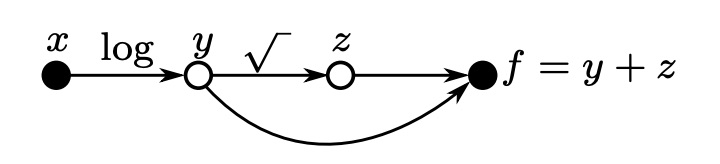
Let’s see another example for the function:

$$f(x)=\frac{\log \left(x+\sqrt{x^2+1}\right)}{x^2}-\frac{{\log }^3\left(x+\sqrt{x^2+1}\right)}{\sqrt{x^2+1}}$$

GIF animation of the computational graph

Final computational graph

We can evaluate $f(x)$ by traversing the graph from the input $x$ to the output $f(x)$.

In PyTorch and other frameworks, the computational graph is constructed when we make the operations, like:

z = torch.sqrt(torch.sum(torch.pow(x, 2),1))

The computational graph gets big very quickly for compelx and highly dimensional functions.

Automatic differentiation: Forward mode

We want to use the computational graph not only to evaluate $f(x)$, but also to evaluate the derivative $\frac{\partial f}{\partial x}$, and w.r.t all the intermediate nodes ($\frac{\partial y}{\partial x},\frac{\partial z}{\partial x}$). We can do that by forward traversing the graph, and compute the derivatives using the other derivatives we compute along the way.

💡 In the forward mode we compute the derivative of the intermediate nodes w.r.t. the input $x$.

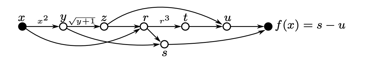
Let’s see how we can compute the $\frac{\partial f}{\partial x}$ by doing the forward-pass on the computational graph of the function $f(x)=\log x+\sqrt{\log x}$.

$$\begin{array}{rl}& \frac{\partial x}{\partial x}=1\\ & \frac{\partial y}{\partial x}=\frac{\partial y}{\partial x}\frac{\partial x}{\partial x}=\frac{\partial \log x}{\partial x}\frac{\partial x}{\partial x}=\frac{1}{x}\frac{\partial x}{\partial x}\\ & \frac{\partial z}{\partial x}=\frac{\partial z}{\partial y}\frac{\partial y}{\partial x}=\frac{\partial \sqrt{y}}{\partial y}\frac{\partial y}{\partial x}=\frac{1}{2\sqrt{y}}\frac{\partial y}{\partial x}\\ & \frac{\partial f}{\partial x}=\frac{\partial f}{\partial y}\frac{\partial y}{\partial x}+\frac{\partial f}{\partial z}\frac{\partial z}{\partial x}=\frac{\partial (y+z)}{\partial y}\frac{\partial y}{\partial x}+\frac{\partial (y+z)}{\partial z}\frac{\partial z}{\partial x}=\frac{\partial y}{\partial x}+\frac{\partial z}{\partial x}\end{array}$$

The assumption we make is that each partial derivative is a primitive, that has a closed form solution and so can be computed on the fly. This is implemented using a lookup table ($O(1)$ cost for the look up) that maps each type of primitive derivative to its closed form solution in order to get the result efficiently.

If the input has only one dimension, than the cost of computing $\frac{\partial f}{\partial x}$ is the same as computing $f(x)$.

In general though, if the input has $p$ dimensions, the cost of computing $\nabla f(x)$ has a multiply factor of $p$, since we have to compute $p$ different derivatives w.r.t all the parameters ($p\times \text{cost of computing }f(x)$ ).

Automatic differentiation: Reverse mode

The solution to compute the gradient of $f$ in an efficient way that doesn’t depend on the input dimensionality $p$ is by traversing the graph in the reverse mode, meaning from the output $f$ to the input $x$, computing all the derivatives of $f$ w.r.t. the inner nodes ($\frac{\partial f}{\partial z},\frac{\partial f}{\partial y},\dots \frac{\partial f}{\partial x}$).

💡 In the reverse mode we compute the derivative of the output $f$w.r.t. the intermediate nodes.

Let’s again see how we can compute $\frac{\partial f}{\partial x}$ of the same function $f$, but this time traversing the graph in the reverse order:

$$\begin{array}{rl}& \frac{\partial f}{\partial f}=1\\ & \frac{\partial f}{\partial z}=\frac{\partial f}{\partial f}\frac{\partial f}{\partial z}=\frac{\partial f}{\partial f}\frac{\partial (y+z)}{\partial z}=\frac{\partial f}{\partial f}\\ & \frac{\partial f}{\partial y}=\frac{\partial f}{\partial z}\frac{\partial z}{\partial y}+\frac{\partial f}{\partial f}\frac{\partial f}{\partial y}=\frac{\partial f}{\partial z}\frac{\partial \sqrt{y}}{\partial y}+\frac{\partial f}{\partial f}\frac{\partial (y+z)}{\partial y}=\frac{\partial f}{\partial z}\frac{1}{2\sqrt{y}}+\frac{\partial f}{\partial f}\\ & \frac{\partial f}{\partial x}=\frac{\partial f}{\partial y}\frac{\partial y}{\partial x}=\frac{\partial f}{\partial y}\frac{\partial \log x}{\partial x}=\frac{\partial f}{\partial y}\frac{1}{x}\end{array}$$

💡 Note that $\frac{\partial f}{\partial y}$ is the sum of the derivatives of the two path on the graph because $f$ is obtained like the sum of $y$ and $z$.

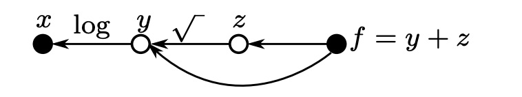
Reverse mode requires computing the values of the internal nodes first, which can be done by doiing a forward pass, in which we just evaluate the function and its inner node, but we don’t autodifferentiate. Once done that, we can do a backward pass in order to compute the derivatives of the output w.r.t. to each inner node and the input.

Forward mode vs Reverse mode computational cost

When we train neural networks, we’ll always have a loss function of the type:

$$\ell :{\mathbb{R}}^p\to \mathbb{R}$$

That maps a $p$ dimensional vector to a scalar. Even if the output of the network has $q$ dimensions, the output of the loss function will always be a scalar.

In a general way, we can write the forward-mode autodifferentiation and the reverse-mode autodifferentiation in this way:

Let ${\mathbb{J}}_k$ be the Jacobian (generalization of the gradient: matrix of partial derivatives) at layer $k$, then:

• Forward-mode autodiff**:**

  $$\nabla \ell ={\mathbb{J}}_{t-1}({\mathbb{J}}_{t-2}(\cdots ({\mathbb{J}}_3({\mathbb{J}}_2{\mathbb{J}}_1))))$$

  The parenthesis in this case defines how we store the operation into a new variable. Each operation that is inside of parenthesis will be stored and then reused in the chain rule.

  In this case (reading from right to left) since the first layer has a dimensionality of $p$, this dimensionality will be carried throughtout all the computation, and so we need to a number of operations more or less equal to:

  $$p\sum _{k=2}^{t-1}{d}_k{d}_{k+1}$$

• Reverse-mode autodiff:

  $$\nabla \ell =(((({\mathbb{J}}_{t-1}{\mathbb{J}}_{t-2}){\mathbb{J}}_{t-3})\cdots ){\mathbb{J}}_2){\mathbb{J}}_1$$

  In this case we start from the last layer, that we know being a scalar, so we will carry out through the computation only the single dimension, and so we need to compute a number of operations that don’t depend on the dimensionality of the input.

  $$1\sum _{k=1}^{t-2}{d}_k{d}_{k+1}$$
  💡 Backpropagation is the reverse mode automatic differentiation applied to deep neural networks.

  Autodifferentiation is a general computational technique that allows to efficiently compute derivatives. This is different from symbolic differentiation (tools like Mathematica) that returns the symbolic formula that describes the derivative.