Convolutional Neural Networks

Convolutional Neural Networks are Feed Forward Networks that use convolution between the image and a learnable kernel in order to extract features, while having only a set of shared parameters to learn (the kernels’).

Feed Forward Network means that the signals goes from start to end, and never goes back (like in autoregressive models, where the output of the model at step $i$ is given in as model input at step $i+1$).

In the first years of CNN development, the deeper the CNN, the better the performances were. This is not true anymore, since very deep CNNs are harder to train, since they suffer from vanishing gradients and other problems.

Even if Transformers are way more powerful on most of the tasks, CNN are still the State of the Art in some modern problems, requiring also less data and less computation w.r.t Transformers.

Why CNNs?

CNNs leverage some properties of the data in order to make the network computation feasable.

Those properties are:

• Spatial locality (or stationarity): statistics of the image are similar at different locations. For example, an eye is an eye in any position in the image, same thing for all the other objects. So to recognize an eye you only need the eye region.
• Compositionality: a table is composed by legs, so recognizing the legs helps in recognizing the table.
• Translation Equivariance: a book upper left is still a book down right.
• Self-similarity: it’s possible recognize two eyes using the same eye-recognizer.

If we want to use a Fully Connected Network for image classification on an image of $1000\times 1000$ we would have $10^{12}$ parameters, which is not feasable at all.

Leveraging the properties listed above, and by having $10\times 10$ kernels, we would have only $10^6$ parameters.

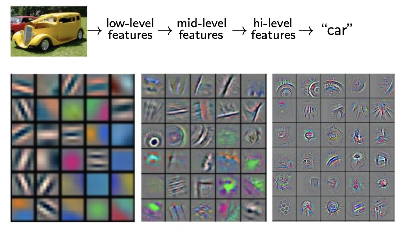
In practice, CNNs will learn multiple filters, each one focusing on some particular set of features.

Convolutional Layer in Detail

In a Fully Connected Layer (not convolutional), the input $x$ has to be flattened ($1\times d_1)$. Then we take the dot-product between a learned matrix $W$ ($d_2\times d_1)$, which will produce a vector of dimensions $1\times d_2$. This because taking the dot-product between a row of $W$ and the input $x$ will result in a single number.

In a Convolutional Layer, we preserve the spatial structure, meaning we don’t have to flatten the input.

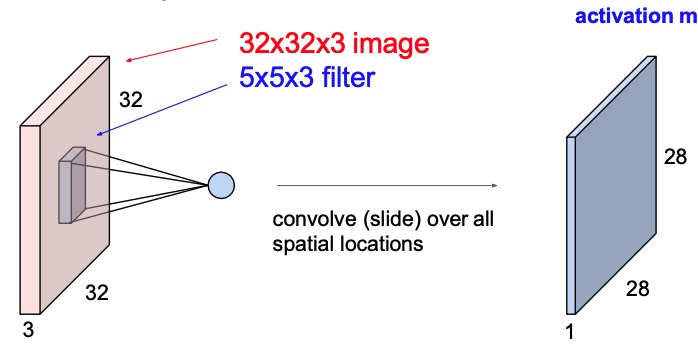
Let’s say we have in input an image $x$ of shape $(32,32,3)$, where $32\times 32$ are the height and width, and $3$ is the number of channels (RGB). Then if we have a filter $w$ of shape $(5,5,3)$, we can convolve it with the image.

We put the filter on the top-left corner of the image, and we output the dot-product plus learnable bias $w^{T}x+b$ between the filter and the image, which will produce a single number. Then we let the filter slide on all possible position, and we map those results into a final activation map. This activation map will have shape $(h,w,1)$ where $h$ and $w$ will be smaller than the original height and width.

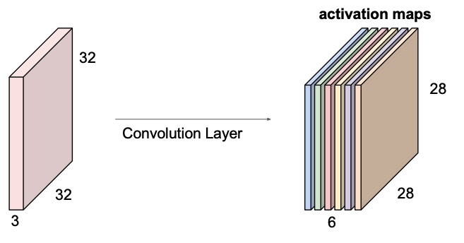
We do that process for each filter we want to learn, wand we stack the activation maps together.

Note

The filter always extend the full depth of the input volume, that’s why the third dimension is $3$, because the input depth is $3$.

A Convolutional Neural Network is just a sequence of Convolutional Layers, between which we put activation functions to insert non-linearity.

At the end you will have some Fully Connected Layers that will take the flattened activation maps and will produce some result. If the task is multi-class classification, the network last layer output shape will be $1\times 1\times 10$, that once softmaxed will output a probability distribution for each class.

The FCN at the end are not mandatory, and we can solve some tasks also only with convolutional layers.

Stride

The stride is defined as the slide step of the filter during convolution. The higher the stride, the lower the resolution of the activation map.

If we don’t want to lower the resolution of the image, we can use a stride of $1$ and pad the images with $0$s. This is not always a good idea since we are introducing some information on the borders, and because of this that particular information cannot be reliable.

In order to compute the activation map resolution, we follow this formula:

$$\frac{(N-F)}{S}+1$$

Where $F$ is the size of the kernel, $N$ the size of the input and $S$ the stride.

Pooling

Pooling is an opeation that aggregates patches of the image into single pixels, in order to reduce the dimensionality of the representations and make the computation more managable.

The main pooling strategies are:

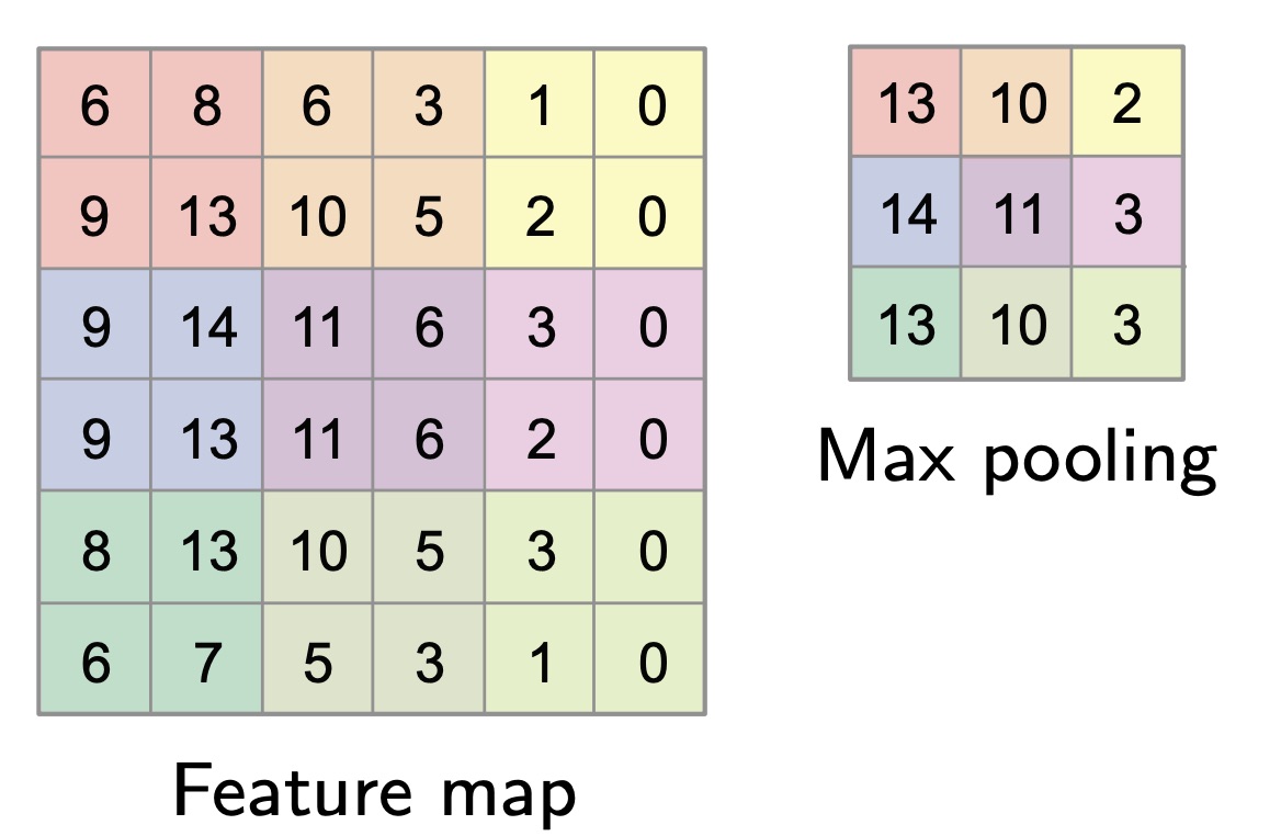
• Max pooling: it takes the maximum of each element of a certain patch;
• Average pooling: it takes the average between the elements inside of a patch.

Note that pooling operates on each activation map independently.

Pooling can be fully replaced by the a stride greater than one.

Receptive Field

The receptive field is the amount of information a certain pixels at level $L$ holds, w.r.t to the original input. If a layer has receptive field of $K$, this means that a single pixels aggregates the information of a patch $K\times K$ pixels in the input.

For convolutions with a kernels of size $K$, each element in the output depends on a $K\times K$ receptive field in the input.

Each successive convolution adds $K-1$ to the receptive field size. This means that with $L$ layers, the receptive field size is $L(K-1)+1$. With that we can deduce that the receptive field increase linearly with the number of layers.

This is a problem, because it means that we need a lot of layers in order to “see” big objects in the image.

If we use stride, we can mitigate the problem, since we are multiplying the receptive field at each layer by $S$ (the stride).

Invariances

A property that may be great to have with CNN is translation and rotation invariance, meaning that the result shouldn’t change if the position of the object in the space and its rotation change.

CNNs are neither translation nor rotation invariance, but they can be trained to be by changing the data.

In order to obtain those invariances, the training set can be augmented with random rotations for the rotation invariances, and with random crops for the translation invariance, since random crops would translate the object of interest in another position.

Notable Architectures

AlexNet

AlexNet is a convolutional neural network architecture that was developed by Alex Krizhevsky, Ilya Sutskever, and Geoffrey Hinton. It was the winning model in the ImageNet Large Scale Visual Recognition Challenge (ILSVRC) in 2012, which marked a breakthrough in the field of computer vision.

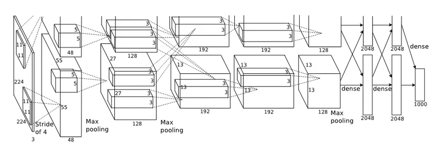
The architecture of AlexNet consists of five convolutional layers followed by three fully connected layers. The convolutional layers use small receptive fields and are followed by max-pooling layers. The activation function used in AlexNet is the ReLU.

One of the notable features of AlexNet is its use of data augmentation (random transformations such as cropping, flipping and rotation to the training images) and dropout regularization techniques, which help in reducing overfitting.

AlexNet also made use of GPU acceleration, which significantly sped up the training process. It was one of the first models to leverage the power of GPUs for deep learning.

Because of the limited resources at the time, the architecture is horizontally split, meaning that they distributed the workload evenly on both the GPUs and then mix the results to obtain the final prediction. If we analyze the visualization of the activation maps for each pipeline, it’s possible to notice that one pipeline learned about grayscale features, while the other one focused more on color schemes.

AlexNet played a crucial role in advancing the field of deep learning and demonstrated the effectiveness of deep convolutional neural networks for image classification tasks.

ResNet

ResNet was the first architecture to be very deep. The first version ResNet architecture was ResNet-34, which had 34 convolutional layers.

In order to solve the problem of the vanishing gradients when dealing with really deep networks, they used Residual Connections (hence the name ResNet), which are skip connections that connect a layer input to the next layer input, without passing through the convolution. The result is then simply added.

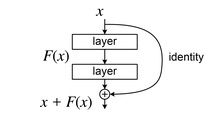
Thanks to the added term, the gradient will always have that term, and so it won’t vanish, meaning that an update to the weights will always be done, and the training will go on.

Visualizing ConvNets

Visualization of deep learning model is crucial to reason about how the models made some choices, in order to improve them and discover new techniques. Interpretation is not always easy though.

Regarding ConvNets, Zeiler et al. proposed a method to map activations at higher layers back to the input, in order to visualize which activation map is responsible for which particular feature directly in the input space.

The process is done by performing the same operations as the Convnet, but in reverse (unpool feature maps and deconvolve unpooled maps). The convnet reverse is called a Deconvnet.

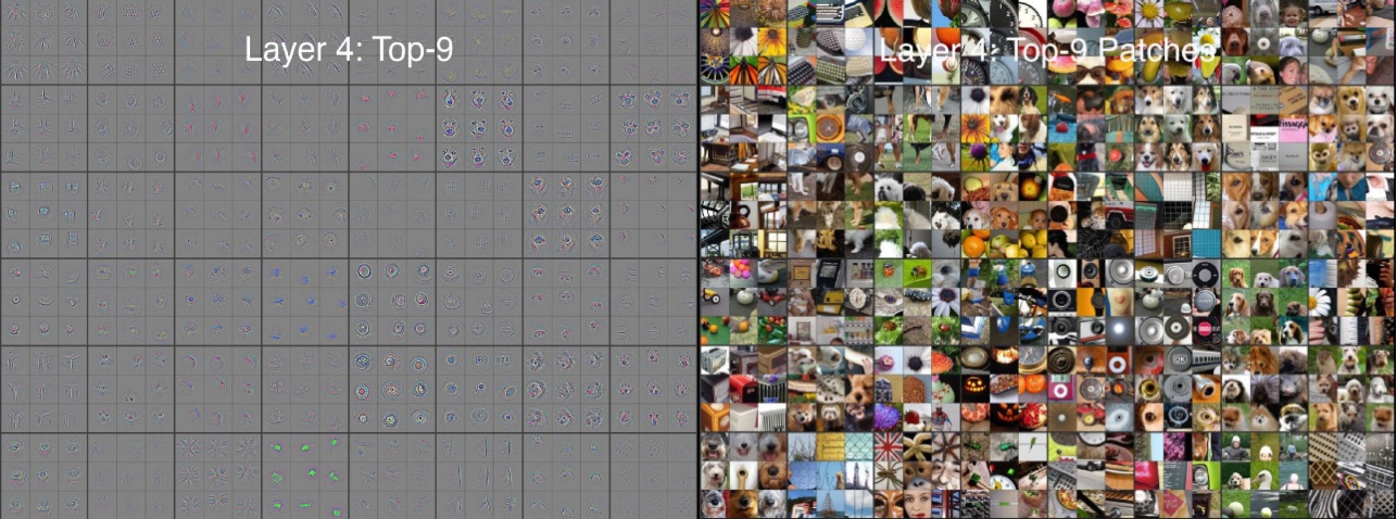
In this image we can see how the learned filters at the 4th layer actually recognize higher level objects in the input image. The features will be at an higher level the deeper the layer in the network (beacuse of the higher receptive field).

Deep Learning Course Definition

Todo

This has to be merged with the above content

Convolutional Neural Networks

What makes Convolutional Neural Networks (CNN) interesting is the fact that they exploit data priors in order to obtain great results with much less parameters than MLP.

Priors

Since deep neural networks can be very complex, have a huge number of parameters and so can be difficult to optimize, we need additional priors as a partial remedy.

For each piece of data that we want to learn, we assume that it has a structure underneath that has to be learned.

Images that are completely random do!n’t have a structure, and so there is nothing to learn. In real world examples images always have some structure, so this can be considered as a prior: structure in terms of repeating patterns, compositionality, locality and more.

Note

For example, if we want to solve a small-piece jigsaw puzzle, where an image is tassellated and each piece is in a random position, we can just rearrange the pieces in order for them to be close to the ones that have the lower jump in color. By doing this, we will obtain the original image.

This of course is valid not only for images, but for every type of data.

Self-Similarity

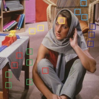
Data tends to be self-similar across the domain. For example in the image above, we can see that patches of pixels, even if they semantically represent different things, are very similar between each other.

This is also true at different scales, meaning that the phenomenon will appear even if we consider larger or smaller patches of pixels.

An example: PatchMatch

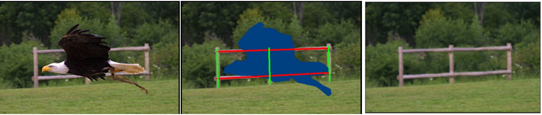
Here we can see an example on applied self similarity. The purpose of the algorithm is to remove the eagle from the image. It works by letting an user drawing a mask that represent the region where the eagle is, and then replacing each region of the mask with the patch (taken from within the image) that is the most similar to the borders of the mask.

Convolution

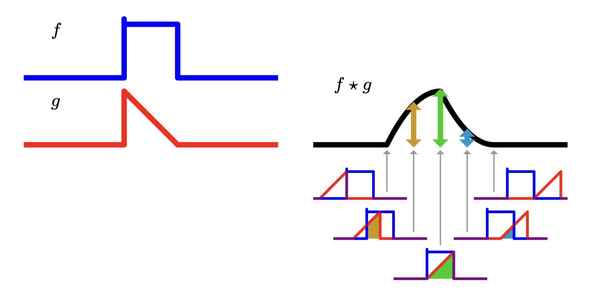
Given two functions $f,g:[-\pi ,\pi ]\to \mathbb{R}$, their convolution is defined as:

$$\underset{\text{feature map}}{\underbrace{(f\star g)(x)}}={\int }_{-\pi }^{\pi }f(t)\underset{\text{filter}}{\underbrace{g(x-t)}}dt$$

Note

The convolutional filter $g$ is also called convolutional kernel in the calculus terminology.

We can image this operation as taking the function $g$, flipping it to obtain $g(-t)$, and then adding $x$ for each possible $x$, that is equal to sliding the function over the function $f$, and taking the element-wise product between the two.

💡 We have $\pi$ in this definition because in case of $f$ and $g$ are signals, we assume that they have a period of $\pi$, but this only in the definition.

Commutativity

Note that convolution is symmetric, meaning that the convolution operator is commutative, so the order of the function doesn’t change the final result.

$$(f\star g)(x)={\int }_{-\pi }^{\pi }f(t)g(x-t)dt\stackrel{z:=x-t}{=}{\int }_{-\pi }^{\pi }f(x-z)g(z)dz=(g\star f)(x)$$

Linearity

We can see convolution as the application of a linear operator $\mathcal{G}$, and so we can define it as:

$$\mathcal{G}f(x)=(f\star g)(x)={\int }_{-\pi }^{\pi }f(t)\underset{\text{filter }}{\underbrace{g(x-t)}}dt$$

It’s easy to show that $\mathcal{G}$ is linear:

• Homogeneity:

$$\mathcal{G}(\alpha f(x))=\alpha {\int }_{-\pi }^{\pi }f(t)g(x-t)dt=\alpha \mathcal{G}f(x)$$

• Additivity:

$$\begin{array}{r}\mathcal{G}(f+h)(x)=\\ {\int }_{-\pi }^{\pi }f(t)g(x-t)dt+{\int }_{-\pi }^{\pi }h(t)g(x-t)dt\\ =\mathcal{G}f(x)+\mathcal{G}h(x)\end{array}$$

And translation-equivariance can be phrased as:

$$\mathcal{G}(\mathcal{T}f)=\mathcal{T}(\mathcal{G}f)$$

Discrete Convolution

Since we have to implement the convolution operation, we need to change the setting from continuous to discrete. We define the convolution as:

$$(\mathbf{f}\star \mathbf{g})[n]=\sum _{k=-\infty }^{\infty }\mathbf{f}[k]\mathbf{g}[n-k]$$

Where $f$ and $g$ are two vectors, and $g$ is the kernel.

2D Discrete Convolution

On 2D domains, for example in the case we are working with RGB images, for each channel the convolution is defined as:

$$(\mathbf{f}\star \mathbf{g})[m,n]=\sum _k\sum _{\ell }\mathbf{f}[k,\ell ]\mathbf{g}[m-k,n-\ell ]$$

We can interpret the convolution as a window (kernel) that slides on each discrete point of the image, and computes the summation as a result.

In matrix notation:

Let:

• $\mathbb{F}$ be the input matrix of size $M\times N$.
• $\mathbb{G}$ be the kernel (filter) matrix of size $\ast K\times L\ast$.
• $\mathbb{H}$ be the output (convolved) matrix of size $(M-K+1)\times (N-L+1)$.

Padding and stride

No padding (no strides)

In case the image is not padded, meaning no values are added on the border, the convolutional kernel is directly applied on the image, and so the result will be smaller, since the kernel can’t go out of the borders of the image.

Full zero-padding (no strides)

In this case the image is padded with zeros in order to compute each single summation, meaning the kernel center point overlaps on each point of the image. This inevitably produces a larger image.

Arbitrary zero-padding with stride

In this case we have just a single “layer” of zero-padding, but we also have a stride of 2, meaning that each time the kernel is moved, we skip one pixel.

CNN vs MLP

Introducing CNNs, we are replacing the large matrices inside of MLPs with small local filters, that are the convolutional filters.

Since we are solving by the numbers inside the convolutional filters, meaning they are the weight that will change according to the loss function, we have much less parameters compared to the MLP.

💡 Because of the fact that the filters change according to the loss function, if the problem is of classifying images that contains eyes to the one that don’t, the filters will probably be very similar to eyes.

This is due also because of the fact that the convolution between the patch and the image is the same as taking the inner product, so if the two matrices are aligned (pointing in the same direction in the space they’re represented, meaning they’re very similar) the inner product will be higher; if they are orthogonal it will be 0; and if they are aligned but with opposite direction, the inner product will be very negative.

So when the kernel, that’s similar to an eye, is convolved on a patch that contains an eye, it will have an high value, and that indicates that that feature is present.

Furthermore, the weights of the convolutional kernels are shared, meaning that they’re present only in the filter, and they’re the same when the filter is convolved with different patches of the image.

The number of parameters also doesn’t depend on the input size, differently from an MLP, since the first linear map has to be the size of the input.

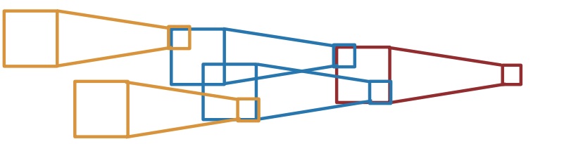
MLP fully connected layer

In a MLP fully connected layer, we have that each input dimension contributes to each output dimension, and so each ouput dimension has a contribute to each input dimensions. Each edge is a different weight, which represent the matrix that we apply at a certain level.

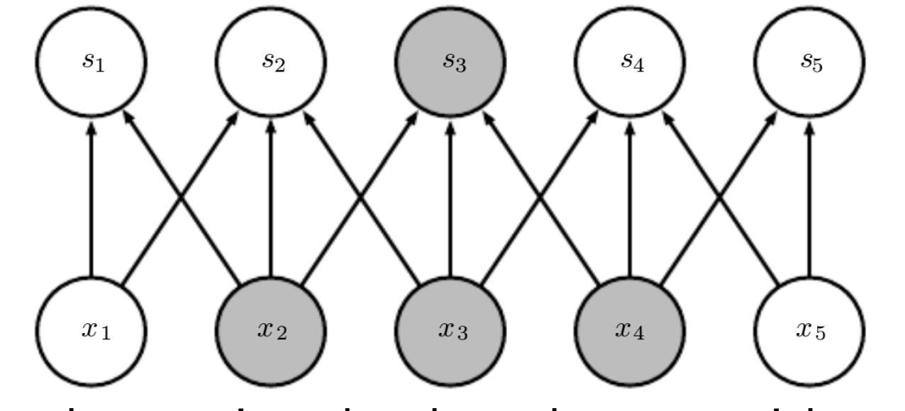
Convolutional layer

In a convolutional layer there are less weights. In this case the kernel size is $3\times 3$, and so each input dimension contributes only to $3$ output dimension. The weight are shared, meaning that the three arrow that exits from each dimension are always the same.

So in this case we have 25 parameters for the MLP and only 3 for the CNN.

Pooling

Since deeper we go into the network, more higher level are the features (meaning they’re closer to the final output), it means that there is some scaling process in the middle.

The scaling process is the pooling operator, which takes non-overlapping patches of the image, and produces another smaller image.

Max pooling for example takes only the max for each patch. This is sensible to noise, since if there is a peak, only the peak will be considered.

Another type of pooling is the average pooling, that returns the average value of the patch.

Pooling allows to capture higher and higher features deeper in the network.