Semantic Segmentation

[!Useful Resources]

• Lecture 11 | Detection and Segmentation

Semantic segmentation is a pixel-wise classification. Meaning each pixel belongs to a certain class.

If there are two cats, their pixels will be identified and classify accordingly.

The thing that differs semantic segmentation to instance segmentation (semantic segmentation + object detection) is the fact that the latter segments the single objects, even if there are multiple instances. For example, if there are two dogs, semantic segmentation will classify those pixels as “dog”, while instance segmentation will also divide the pixels of one dog from the one of the other.

Things vs Stuff

• Things are countable objects that can have individual instances with separate identities, such as people, animals, tables, pens.
• Stuff is something that doesn’t have a shape and a notion of instance, such as the sky, the forest.

An aggregation of things can make a stuff, for example multiple threes make up a forest.

Semantic Segmentation Ideas

Sliding Window

This approach consists in taking a patch of an image and classify the center pixel using a CNN. The rest of the pixels will be used as context. The patch is then moved in order to classify all the pixels.

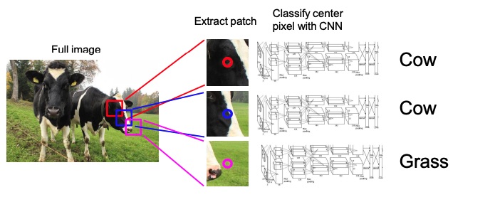
This is very inefficient since we are not reusing the shared features between the overlapping patches.

Fully Convolutional

In order to make the method more efficient, we can design a network as a bunch of convolutional layers with zero padding and a stride of 1 in order to maintain the spatial resolution to make predictions for the pixels all at once. The scores will be $C\times H\times W$ with $C$ being the fixed number of classes we’re interested in (we know that from the dataset).

Each $1\times H\times W$ contains the score of each pixels belonging to that particular class.

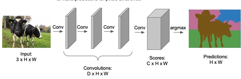
The problem is that the convolutions at the original image resolution will be very expensive, since in the middle layers you would have many channels, from $64$ to $256$, with a huge resolution.

In order to avoid that, we can downsample the image at the beginning of the network and upsample it at the end of the network. The downsampling part is very similar to CNN used for image classification, but then instead of transitioning to a fully connected layer, we upsample the image to its original resolution in order to get the masks.

In most of these types of networks the downsampling and upsampling is symmetrical.

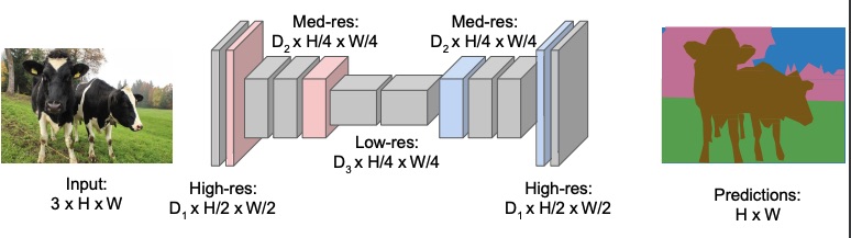
Regarding the downsampling, we can achieve that in the classical ways, such as with pooling or strided convolution.

On the other hand, it’s not clear how we can achieve upsampling.

Upsampling Techniques: Unpooling

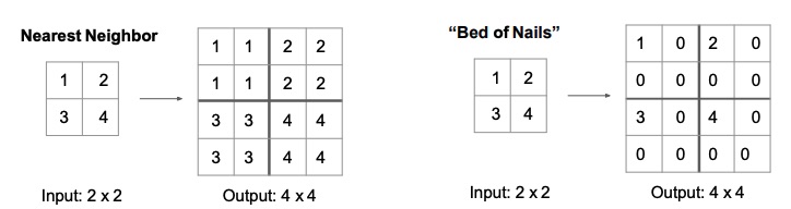
The unpooling operation tries to revert the result of the pooling operation loosing as little information as possible.

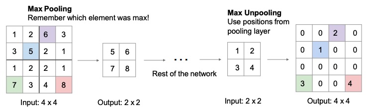
The most naive techniques are Nearest Neighbours, which just replicates the value $n$ times in order to get to the original dimensionality; and Bed of Nails, which replaces all the other values with $0$ and puts the current value in the just one region square obtained by each expansion, in the figure below that region is the upper-left corner.

A smarter way of unpooling is Max Unpooling, which can be applied as the reverse of Max Pooling. The idea is to remember in which position in the original matrix the value was, and to place it back in that position when using an unpooling technique similar to bed of nails.

The problem with all these techniques is that we will lose a lot of information regardless.

Learnable Upsampling: Transpose Convolution

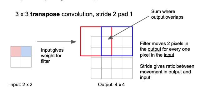
The idea behind transpose convolution is to convolve the input with a learnable kernel, and to produce an output that is bigger than the input, by moving it two pixels in the output for every pixel in the input. We just take the sum where the output overlaps.

Instead of taking the dot product between the kernel and the patch, we get the pixel in the image at position $(i,j)$, we then multiply that scalar value with the kernel, and then copy that value over that $K\times K$ region in the upsampled image, where $K$ is the kernel dimension. Where two kernel positions overlap we just sum the values.

The input is used as a weight that weights the convolutional kernel. So the outputs will be weighted copies of the filter. Here the stride gives the ratio of the output with respect to the input. So a stride of $2$ will produce a bigger upscaling, since we’re moving $2$ pixels in the output for every one pixel in the input.

Note

Remember that in the standard convolution the stride tells the ratio of the input w.r.t. the output.

Below there is also an example of a 1D transpose convolution. As we can see each kernel element is weighted by the input and then copied on the output. The overlap is then summed.

The sum can be a problem since it might produce some checkboard artifacts in the output, because the more the upsampling layers, the higher the magnitude of some elements. Because of that, a kernel of $4\times 4$ or $2\times 2$ both with a stride of $2$ instead than a $3\times 3$ with a stride of $2$ can be helpful.

Convolution as Matrix Multiplication

In order to be more efficient we can express the convolution as a matrix multiplication operation, which is what is done in most of the popular deep learning frameworks.

$$\vec{x}\ast \vec{a}=X\vec{a}$$ $$\left[\begin{array}{cccccc}x& y& z& 0& 0& 0\\ 0& x& y& z& 0& 0\\ 0& 0& x& y& z& 0\\ 0& 0& 0& x& y& z\end{array}\right]\left[\begin{array}{c}0\\ a\\ b\\ c\\ d\\ 0\end{array}\right]=\left[\begin{array}{c}ay+bz\\ ax+by+cz\\ bx+cy+dz\\ cx+dy\end{array}\right]$$

If we want to do a strided convolution, let’s say stride of $n$, we can just keep one line for each $n$ lines.

$$\left[\begin{array}{llllll}x& y& z& 0& 0& 0\\ 0& 0& x& y& z& 0\end{array}\right]\left[\begin{array}{l}0\\ a\\ b\\ c\\ d\\ 0\end{array}\right]=\left[\begin{array}{c}ay+bz\\ bx+cy+dz\end{array}\right]$$

Transpose Convolution as Matrix Multiplication

The name Transpose Convolution comes from the fact that if we transpose the $\vec{x}$ for the strided convolution and replace the $a$ accordingly, we obtain an upsampled vector.

$$\vec{x}{\ast }^T\vec{a}=X^T\vec{a}$$ $$\left[\begin{array}{cc}x& 0\\ y& 0\\ z& x\\ 0& y\\ 0& z\\ 0& 0\end{array}\right]\left[\begin{array}{c}a\\ b\end{array}\right]=\left[\begin{array}{c}ax\\ ay\\ az+bx\\ by\\ bz\\ 0\end{array}\right]$$

Evaluation Metrics for Semantic Segmentation

Segmentation is a pixel classification, and since most of the time 99% of the object is not the interest object (sky and 1% birds), if we classify everything as sky we will have 99% accuracy. This is why accuracy is not suited as an evaluation metric.

A good approach is Intersection Over Union, meaning we take the intersection between the ground truth segmentation and the computed segmentation, and we divide it by the union. The maximum score is $1$.

Segmentation Data Collection

Data collection is a nightmare for segmentation, since the annotator needs to be very accurate when annotating pixels. A common thing is to annotate few classes and mark the rest as “other”. A single HD image may take 1 to 2 hours to annotate precisely.

There are some tools that allow a semi-automatic labelling annotation, meaning that it shows to the user many ways to segment a region and the user just has to choose one. Others allows the user to annotate only some pixels and the model will do the rest. This speeds up the process.

The most common dataset for training and benchmarking segmentation models is COCO (Common Objects In Context), with a collection of around 300K images (200K of which are labelled) within 80 object categories and 91 stuff categories.