Gradient descent is an iterative algorithm that allows to find the minimum of a certain function. This is useful in order to find the parameters that minimize a certain loss function that cannot be solved analitically.
The algorithm uses tha fact that the gradient of a function is a vector defined of the domain of the function which encodes the direction of its steepest ascent. This mean that we should be able to follow the direction of the negative gradient at each point in order to go towards the minimum of the function.
The general idea is:
- Start from some point ;
- Iteratively compute the at the next step:
- Stop when the minimum is reached.
We can write the formula in this way:
Remember that is possible to perform the subtraction because the gradient of the function lives in the domain of the function, and so the dimensionality will match.
In order to visualize the gradient, assuming , we can both visualize the 2D function in a 3D space, or we can inspect its iso-lines.
An iso-line (or level curve) is the line of the function projected into the plane where the function has the same value. Each function has infinitely many iso-lines. Note that an iso-line is always a closed path.
This is useful since we can see the gradient as a vector field in a 2D surface.
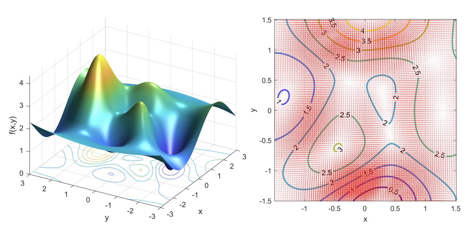
The 2D function and some of its iso-lines
We can zoom on the iso-lines in order to better inpect the negative gradient.
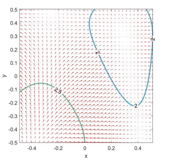
From this image we can see that the vector field is smooth, that’s because the function is smooth. Also we can notice that the arrows points towards a lower zone of the function, that’s because we are dealing with the negative gradient.
The gradient in each point has different direction and magniture.
This representation is also valid for 3D functions, meaning . In this case the projection of the function will be a surface, and so they will be called iso-surfaces (or level surfaces).

Orthogonality of the gradient
From the 2D gradient vector field, we can also notice that each arrow on the iso-line is orthogonal to that line. Since there are infinitely many iso-lines, each arrow is orthogonal to a certain iso-line.
The proof is done by introducing the concept of directional derivative, that is the derivative of a multidimensional function with respect to a certain vector in that space. The vector encodes also the direction.
This because in a 1D function we can only compute the derivative in two directions, but in a 2D (or more) function we have infinitely many directions in which we can compute the derivative.
The directional derivative of the function with respect of the vector is written as , and it’s equal to the inner product between the gradient and the vector.
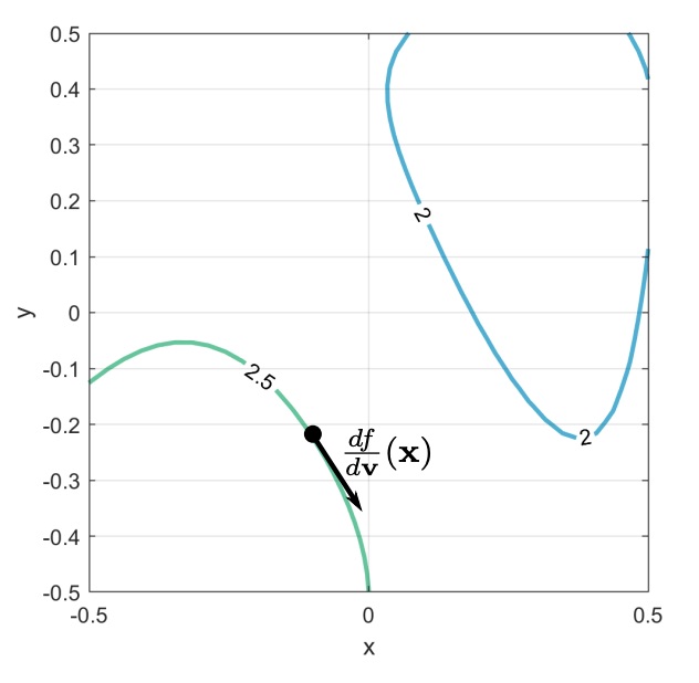
The directional derivative will be a vector tangent to the iso-line, and by definition the iso-line is made out of the points in which the function has the same value, and so in that direction the value won’t change. This means that the derivative is zero, and so the inner product also is zero.
The fact that means that is orthogonal to , and so is orthogonal to the iso-line.
Differentiability
In order to apply gradient descent the function must differentiable.
For a function in 1D being differentiable means that we can compute its derivative. For a function with more dimensions, if we can compute all its partial derivatives doesn’t mean that the function is differentiable.
is differentiable only if it has a continuous gradient.
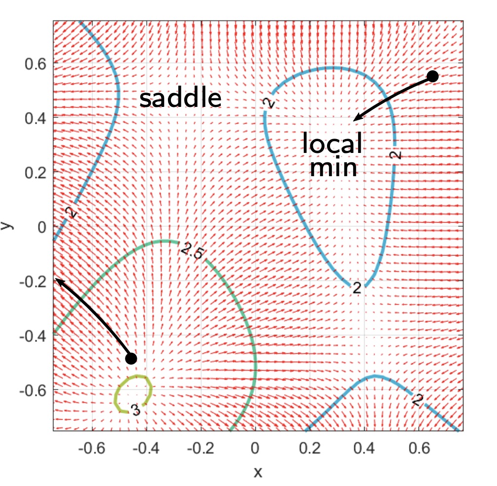
Stationary points
A stationary point is a point in which the gradient tends to zero. Gradient descent “gets stuck” at stationary point.
These points can be part of a local minimum or a saddle point.
Gradient descent will always end up in a stationary point, which stationary point depends on the initialization point.
In general we don’t want to find the global minimum of the function, since this would lead to bad performances (overfitting), but if you really want to optimize a function you can perform gradient descent with a lot of different initialization point, get to the same amount of minima, and then get the minimum of those minima.
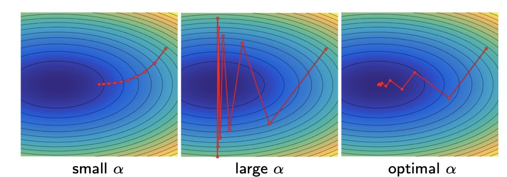
Learning Rate
The parameter is called learning rate in the machine learning field, because it allows to scale up or down the step that we take on each iteration. Note that is not the step, but is.
A small means that we take small steps in the direction of the steepest descent, and so we will surely end up into a stationary point, but it may take a while.
A large means that we take big steps, which means that we might arrive to the minimum faster, but we also risk to overshoot it, meaning we always surpass it because the step is too big.
Another way is to find the optimal by a line search algorithm. This algorithm uses the fact that we can fix a direction and then solve the equation of the gradient in that direction, that would be 1D, in order to find the best . Formally we want to find .
Decay
Since a big learning rate is good at the start in order to speed up the descent, but it’s bad when the point is near the minimum because of the risk of overshooting, a good idea could be to make the dynamic.
We call this type of adaptive. This is done by decreasing it according to a decay parameter , which defines the rate of the decay.
Examples of functions used to implement the decay are:
This function makes the learning rate decay according to an hyperbolic behaviour, because of the factor.
With this function the learning rate decreases exponentially.
This function linearly scales the learning rate starting from to when the iterations increase.
Momentum
With momentum we mean an extension of gradient descent in which we modify the trajectory of the point by accumulating past gradients.
The momentum is defined as:
Where is (another) hyperparameter that affects the strength of the momentum, and so the acceleration of the point.
We can use the momentum to define the extended gradient descent:
We can re-define the step that we take at each iteration as:
We can see that the step is proportional to and inversely proportional to .
The step length would be maximized when the new gradient has the same orientation as the previous one. This means that the point will accelerate, differently from standard GD in which the “speed” of the descent is always the same.
The physics interpretation of momentum can be thought like a ball that is put on the starting point of a surface. It will descend the surface according to gravity, but because of momentum it won’t change the direction instantly, but after some time.
With momentum the direction of each gradient is not orthogonal to the function iso-lines anymore.
Momentum is useful because it allows to speed up the descent in case the direction is unchanged, it also reduces the noise in case there are multiple changes of orientations, and also makes the point able to escape from local minima that aren’t strong enough.
This because, as a ball will surpass a small bump, the same will happen with a point that goes in a not so deep minimum. In case the point will go on a deeper minimum and doesn’t have too much momentum, it will stay there and stabilize after some time.

Difference between GD with a fixed number of iterations with and without momentum.
First-order acceleration methods
We can unroll the gradient descent, meaning we iterate over the steps and we write down the expression. We can see that in the general case, we can define the as:
-
Unrollment process
And with the use of momentum:
In a more general case, we can see that the gradient inside the summation is being multiplied by a certain coefficient. We can call this coefficient and so we can rewrite the expression as:
So in the case of momentum, we have .
Instead of just multiplying the gradient by a vector, and so scaling it by a certain factor, we also may want to apply some transformation to it. This can be done by multiplying a matrix , and so the even more general equation becomes:
These variations of gradient descent are called first-order acceleration methods, and they differ from each other because of a different matrix. Examples of this optmiziation algorithms are Adam and AdaGrad.
Stochastic gradient descent
Gradient descent requires to compute the loss over training examples, which requires computing the gradient for each term in the summation.
In real world problems, can be very big, and also the number of parameters that we have to optimize, hence the dimensionality of the gradient, can be very big (order of millions). This can scale very quickly.
The idea is to not compute the loss for every single example, but randomly take a subset of a fixed size from the training set , for example , that takes the name of mini-batch .
Even if the dimensionality of the gradient remains unchanged, we just have to do a limited and fixed number of operations on the small set.
This means that we will approximate the gradient for each point, and so the step we take won’t be orthogonal to the iso-lines of the function anymore. Furthermore, if we plot how the loss changes during the various iterations, the curve won’t be monotonous anymore, since sometimes we might take the step in the wrong direction because of the approximation.
Another thing to consider it that we won’t ever stop at the point of minimum, but the point will always oscillate around it because of the noise that is introduced by the random sampling.
Even after this approximation the result is very good, and the speed up with respect to the vanilla GD is significant.
Once we’ve sampled all the examples in taking small mini-batches each time, we have an epoch. The algorithm proceeds for many epochs.
SGD Computational Cost
Let be the number of training examples and the number of parameters (dimensionality of the gradient).
Let also and be two costants related to the conditioning of the problem.
Let also be the accuracy of the approximation with respect to the true value of the loss with the optimal minimizer:
We can prove that the computational cost of the SGD and the GD is the following:
| Cost per iteration | Iteration to reach | |
|---|---|---|
| GD | ||
| SGD |
From this table we can see that SGD is better than standard GD because of many reasons:
- It doesn’t depend on the number of examples;
- It assures the convergence to a minimum in a finite number of steps, differently of GD which can take infinitely many steps before converging to a certain minimum. (WHY THIS?)