Multi Layer Perceptron

A multilayer perceptron (or deep feed-forward neural network) can be seen as a deep nested composition of functions, with a non-linear function (activation function) that produces the output of each single layer.

$$\text{output}\leftarrow (\sigma \circ f)\circ (\sigma \circ f)\circ \cdots \circ (\sigma \circ f)(x)\leftarrow \text{input}$$

Note that the function composition operator $\circ$ is associative, so parentheses are not actually necessary.

$\sigma$ denotes the activation functions. If we have just one layer with the logistic function, then we have the logistic regression model. In general the $\sigma$s will be different across the layers, and can be of various types.

A popular sigma is the ReLU (Rectifier Linear Unit) that is defined as

$$\sigma (x)=\max \{0,x\}$$

And note that this is a continuous function but it has a discontinuous gradient in the point $0$, since on the left of that point the derivative is $0$, and on the right is $x$. So exactly in that point we have a singularity. This means that if the ReLU is present in any layers, the function will be non differentiable, and so we have to take care of it.

Hidden layers

Let’s rewrite the composition of functions $g_{\Theta }(x)$, defined as:

$$g_{\Theta }(x)=(\sigma \circ f_{{\Theta }_n})\circ (\sigma \circ f_{{\Theta }_{n-1}})\circ \cdots \circ (\sigma \circ f_{{\Theta }_1})(x)$$

Each set ${\Theta }_i$ is the set of parameters of the $i$-th layer. Each intermediate layer can be expressed as:

$$x_{\ell +1}={\sigma }_{\ell }({\mathbb{W}}_{\ell }{x}_{\ell }+b_{\ell })$$

Where $\ell$ denotes the layer, $\mathbb{W}$ is the matrix of weights ($\Theta$), $x$ is the input vector to the layer and $b$ is the bias. Sometimes the bias can be included inside the $\mathbb{W}$ matrix, but in this case we must add a dimension full of $1$s in the $x$ in order to match the shapes.

Neurons

Each row of the weight matrix $\mathbb{W}$ is called a neuron or a hidden unit.

$$\mathbb{W}x=\left(\begin{array}{c}-\text{ unit }-\\ ⋮\\ -\text{ unit }-\end{array}\right)\left(\begin{array}{c}\mid \\ \mathbf{x}\\ \mid \end{array}\right)$$

💡 In some papers the *neuron* might refer to the output of the $\mathbb{Wx}$ matrix multiplication.

We can see the matrix multiplication $\mathbb{W}x$ as a collection of $q$ vector-to-scalar functions ${\mathbb{R}}^p\to \mathbb{R}$ made in parallel, resulting in a new ${\mathbb{R}}^q$ vector.

Single layer illustration

A single layer may be illustrated also with a graph where the first layer represents the components of $\mathbf{x}$, the second layer represents the output of the product $\mathbf{Wx}$, that is the linear combination between the vector $\mathbf{x}$ and the $i$-th row ${\mathbf{w}}_i$ of $\mathbf{W}$. We can see that the neuron will be a fully connected with the inputs, this is a fully connected layer. (There will also be cases of non-fully connected layers)

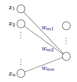
A graph of the fully connected layer

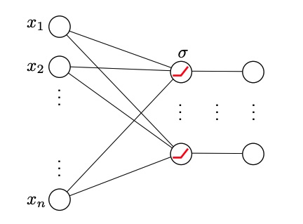
Adding the non-linear function $\sigma$

Output Layer

The output layer determines the co-domain of the network. For example if $\sigma$ of the last layer in the network it’s the logistic sigmoid, then the entire network will map:

$${\mathbb{R}}^p\to (0,1{)}^q$$

That might be a good idea in case of classification, but in a more general case it’s commont ot have a linear layer $f$ at the end of the network in order to map:

$${\mathbb{R}}^p\to {\mathbb{R}}^q$$

Universal Approximation Theorems

There is a class of theorems called Universal Approximation Theorems (UAT) which answers to the question: “What class of functions can we represent with a MLP?

One of the first ever theorems of this class, if not the first one, tells us that:

If $\sigma$ is sigmoidal, then for any compact set $\Omega \subset {\mathbb{R}}^p$, the space spanned by the functions $\varphi (x)=\sigma (\mathbb{W}x+b)$ is dense in $\mathcal{C}(\Omega )$ for the uniform convergence. Thus, for any continuous function $f$ and any $ϵ>0$, there exists $q\in \mathbb{N}$ and weights s.t.:

$$|f(x)-\sum _{k=1}^q{u}_k\varphi (x)|\le ϵ\text{for all }x\in \Omega$$

Being dense in $\mathcal{C}(\Omega )$ it means that if we take all linear combinations of $\varphi$, they allow to represent all the possible continuous functions in a $p$-dimensional euclidean space.

Said that, the theorem tells us that we can approximate each continuous function with the desired accuracy using a MLP that has as few as just one layer. The larger is $q$, the smaller can the error between the real function and the approximator be.

Note that taking linear combinations of all the $\varphi (x)$ means to just add a final linear layer.

There are also other UAT theorems that extends the universality for other $\sigma$s.

From this theorem we could think that a single hidden layer MLP is everything we need since it can approximise every existing continuous function, but we actually can’t. That’s because the theorem just says that those MLPs exist, but doesn’t tell us anything on how to do it.

MLP Training

Given a certain loss ${\ell }_{\Theta }$, solving for the weights $\Theta$ is referred to as training.

In linear and logistic regression problems we’ve seen that the loss was always convex, but in general this isn’t the case. In fact the convexity of the loss comes from how $g_{\Theta }(x)$ is made. So if the neural network approximates a function that is very non-linear and very complex, the loss probably wouldn’t be convex, and so we cannot compute the gradient and set it to $0$ in order to minimize.

Also remember that we don’t want to find the global optimum, otherwise we will risk to overfit the training data.

💡 The loss is convex for very specific cases, for example:

• Linear Regression: One layer, no activation function, MSE loss;
• Logistic Regression: One layer, sigmoid activation, logistic loss.

Note also that the dimensionality of the gradient of $\Theta$ is determined by the dimensionality of the output of $g$.