Temporal Convolutional Networks (TCN)

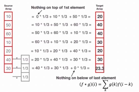
As said before, CNNs work with static data, but it’s possible to extend them in order to make them work with sequential data. Between all the sequence model, this is surely the most efficient one, and in some domains the result are interesting.

In 1D convolutions, let’s say we have a kernel of size 3. This kernel always process 3 inputs, and produces an output.

What this kernel could do, it predict the position at the 4th step, by seeing the first three steps.

The first problem is that CNN accept a fixed-size input, and when we’re dealing with sequences, the length of the sequence may vary.

The second problem with CNN is that they are only able to output a single choice from a fixed list of options, in a $C$ way multi-classification manner. This can be solved by predicting one output at the time.

These types of model are not suited for predicting future words or future motions. This because for example in the picture below, if the kernel is centered on represent, it’s also looking at the future word, and so it can just copy the next word, and it wouldn’t learn.

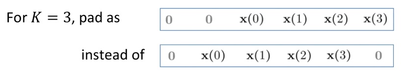
In order to solve this problem, we need the CNN to become casual, meaning that it just has to look at the past inputs.

It’s possible to achive this by just padding asymmetrically, adding the padding only at the $K-1$ initial starting positions, where $K$ is the kernel size.

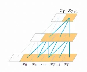
With this kind of architecture, where there are some convolutions between the first and the last layer, and all convolution are causal, the model is able to look at $T+1$ words in the past ($0$ from $T$), and predict the word at step $T+1$.

The input would always be $T+1$ long, since that is fixed. In order to each time predict the next word, we just slide the kernel one word at the time.

In the period when the paper was released, there was a lot of study in RNNs and LSTMs, and the researchers of this paper showed that you can achieve very similar performances with just a convolutions.

This architecture is trivial to parallelize, because the model doesn’t have a memory, and the output at $T+1$ only depends on the inputs $0$ to $T$. For this reason, I can parallelize the kernel on multiple subsequences of the original sequence.

The model is autoregressive, meaning I feed the generated next word into the next step prediction. This is done during inference, but during training it takes the words from the ground truth in order to parallelize the training by processing all the subsequences (taken all the possible positions of the sliding window) in parallel.

Since it’s convolutional, the model also exploits local dependencies.

The problem is that the relationship between the receptive field and the number of layers is linear, meaning that for long term dependencies there is the need of many layers.

In order for the output to depend on the previous $N$ words, you need to solve $1+L(K-1)=N$, where $K$ is the kernel size and $L$ is the number of layers. The relationship is linear. Since usually kernels are small, we would prefer to insert more layers, but this requires more computational power.

A way to solve this problem is to not compute all the operations, but leave some gaps.

Dilated Convolutions

The most naive way to try to solve this problem is to not compute all the operations, but leave some gaps. Let’s say you want an input of size $1000$ without having to put $500$ layers, we can just ignore some input positions.

This can be done with dilated convolution, where each convolutional kernel has the same weights, but considers only one value each $d$ values, where $d$ is called a dilation factor.

Inserting directly some gaps by putting a $d>1$ in the first layer is not a good idea, since some inputs won’t be considered, which may be crucial for the prediction.

A better way of using dilated convolutions is to choose the dilation factor as $d=2^l$ where $l$ is the current layer (starting from 0).

In this way we won’t have any gaps, and so the output would still be a function of all the points in the input.

With this solution, the relationship between the number of layers and the receptive field is logarithmic instead of linear.

Note

This isn’t like stride, since a stride of 2 it means you consider one position and then move by 2., while here the kernel move in the same way, but it’s dilated, meaning it considers only one value each $d$ values. This also doesn’t change the output size like stride.

The dilated kernel are dilated, meaning there one each $d$ elements is considered inside of the kernel. This number is called dilation factor $d$. In the first layer is $d=1$, in the second $d=2$ and in the third is $d=4$. This number is computed as $d=2^l$, where $l$ is the current layer.

Adding residual connection

Taking inspiration from ResNet, which uses residual connection to improve the capability of the model to learn, we can add also here some residual connections.