Fundamentals of Data Science

Todo

This has to be divided in different pages

Introduction

Data

The most difficult part in getting the data needed for making some decision or, in a more general way, doing something useful with it, is to process it and remove the “impurities”, such as misleading data, incorrect data and non-coherent data. The data polishing can get up to 80% of the work in a problem.

Correlation and Causation in Data

Correlation means that two or more variables have some type of relationship.

Causation indicates that one event is the result of the occurrence of another event, in other words, there is a casual relationship between the two events.

Correlation doesn’t imply causation. Correlation is easy to test but causation is almost impossible. A and B are correlated because some C exists such that C → A and C → B.

Example: Every time they light up the belt signal on the plane, it gets bumpy. The light signal and the bumpiness are correlated, but the light signal is not the cause of the bumpiness.

Underfitting and Overfitting

• Underfitting means that models used for predictions are too simplistic. For example 60% of men and 70% of women respond well to an advertisement, so all future ads should go toward women.
• Overfitting means that models used for predictions are too specific. For example if a furniture item has four legs 100cm long with decorations and a flat polished wooden top then it’s a dining room table.

Regression

Regression is used to create a line of best fit for a particular set of points, and use that line as a model to predict new values for new points.

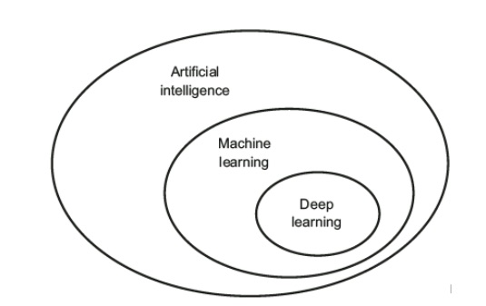
Machine Learning

Machine learning is the field of study that allows computers to learn without being explicitly programmed. The computer is trained with some data and can predict new things with data that has never seen. A computer program is said to learn from an experience $E$ with respect to some task $T$ and some performance measure $P$, if its performance on $T$, as measured by $P$ improves with experience $E$.

• The experience $E$ is modelled by the Data and the Labels
• The task $T$ is modelled by the the activity recognition
• The performance measure $P$ is the accuracy of the prediction/solution

Computer vision

Computer vision is an application of machine learning that tries to solve the inverse graphic problem. For example how to recognize an image from an array of numbers, instead of graphics which problem becomes how to generate an array of numbers that can be translated as an image.

Studying how we humans see the world is not enough to develop a method to make a computer see. It’s useful to compare the biological and technological methods to see why one works and the other doesn’t.

Computer vision can recognize and classify an object starting from an array of grey scale numbers only if it has some more data which it can learn from.

Humans also need data to recognize objects in pictures and interpret depth and perspective. The data in this case is all the images that they’ve seen during their lives. A 2-year-old kid is estimated to see about 80 million images.

Object Identification vs Classification

• Object identification: recognize a certain object, such as your laptop or the apple that you just bought.
• Object classification: recognize that an object belongs to a certain class, such as recognizing any laptop or any apple. This is also defined as “basic level category”.

Once the object is recognized, there are two other operations:

• Segmentation: meaning the separation of the pixels belonging to the foreground (the object) and the background. For example, mark all the pixels that belong to a person inside of an image.
• Localization or Detection: detecting the position of the object in the scene, such as orientation, scale, size and 3d position.

An example of classification

Basic-Level Categories

Inter-class vs Intra-class variation

• Inter-class variation is low when two objects of different classes of objects (inter) are very similar (such as a cow and a dog that looks like a cow).
• Intra-class variation is low when two objects of the same class are very different (such as two different species of dog)

Digital Image Filtering

Image filtering means applying some function to a part or to the entire image.

Image filtering is used for numerous purposes, such as noise reduction, filling in missing information, or extracting image features.

When an image is filtered, the noise may be reduced and so it’s easier to extract useful information, such as known patterns.

Linear Filtering

The simplest filtering is linear filtering, consisting in replacing each pixel with a linear combination of its neighbors. This can be achieved with an operation called convolution.

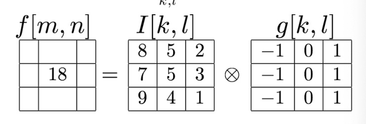
Convolution

Let $I[m,n]$ be the discrete image represented by a matrix Let $g[k,l]$ be the filter “kernel”

The filtered image is the result of the convolution between the Image and the Kernel.

$$f[m,n]=I\otimes g=\sum _{k,l}I[m-k,n-l]g[k,l]$$

$I[m-k,n-l]$ is the same to applying $I[m+k,n+l]$ with the mirrored filter.

We can also have a one dimension filtering, meaning it will be represented as $g[k]$.

Note

Basic properties of Linear Systems

• Homogeneity: $T[aX]=aT[X]$
• Additivity: $T[X_1+X_2]=T[X_1]+T[X_2]$
• Superposition: $T[a{X}_1+b{X}_2]=aT[X_1]+bT[X_2]$
• Linear systems $⟺$Superposition

Filtering to Reduce Noise

Noise is something that we’re not interested in. Is defined as low-level noise the fluctuations of the light, the sensor noise, quantization effects, etc.

Complex noise instead is, for example, shadows and extraneous objects.

Additive Noise

Additive noise is a model that recreates an image applying the following formula: $I=S+N$ where $S\text{, }N\text{, }$ and $I$ are respectively the Signal, the Noise, and the Image.

Note that the noise doesn’t depend on the signal.

Average Filter

This type of filter works by replacing each pixel with an average of its neighbours.

Average filters are useful to reduce the noise of an image since averaging an area (smoothing it) makes it more homogeneous.

When smoothing a little bit of signal (information contained inside the image) is lost. The more the image is noisy, the more smoothing is needed.

Box filter

The simplest of these types of filters weights all the neighbours in the same way.

All the values in the kernel have the same value and add up to 1. An example of a kernel is

$$\frac{1}{9}\left(\begin{array}{ccc}1& 1& 1\\ 1& 1& 1\\ 1& 1& 1\end{array}\right)$$

Gaussian filter

Different from the box filter, this type of filtering weights the nearest neighbours more than the distant ones.

The kernel depends on the $\sigma$ (standard deviation) value, but its central values are bigger than the values on the borders. An example is

$$\frac{1}{16}\left(\begin{array}{ccc}1& 2& 1\\ 2& 4& 2\\ 1& 2& 1\end{array}\right)$$

Smoothing an image with a Gaussian filter instead of a Box filter makes the general details of the image more visible, when smoothing an area weighting all the pixels, in the same way, may lose some details.

When the $\sigma$ is larger, the kernel gets larger and the image is smoother, and vice versa otherwise.

The Gaussian distribution in 2D is represented by the following equation

$$G(x,y)=\frac{1}{2\pi {\sigma }^2}\exp (-\frac{x^2+y^2}{2{\sigma }^2})$$

The Gaussian distribution in 1D is represented by this equation

$$G(x)=\frac{1}{\sqrt{2\pi }\sigma }\exp (-\frac{x^2}{2{\sigma }^2})$$

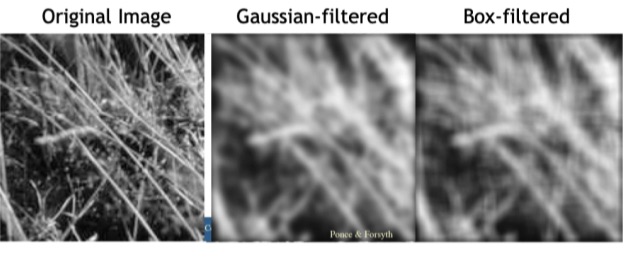
Differences between Gaussian and Box filtering

Separability principle

Both the Box filter and the Gaussian filter are separable, meaning they can be written as the product of two or more simple (lower dimension) filters.

This is an example of the separation of a 2D Box filter.

$$f_x\otimes f_y=\left(\begin{array}{ccc}\frac{1}{9}& \frac{1}{9}& \frac{1}{9}\\ \frac{1}{9}& \frac{1}{9}& \frac{1}{9}\\ \frac{1}{9}& \frac{1}{9}& \frac{1}{9}\end{array}\right)=\left(\begin{array}{ccc}\frac{1}{3}& \frac{1}{3}& \frac{1}{3}\end{array}\right)\otimes \left(\begin{array}{c}\frac{1}{3}\\ \frac{1}{3}\\ \frac{1}{3}\end{array}\right)$$

💡 Gaussian separability demonstration is on page 98 of [slide 2](https://drive.google.com/drive/folders/1H7keN8wz8L9AFMr60oWKVgsLi-YYDD5Z)

As the demonstration shows, generally a filter is separable if you can factorize its equation, which depends on $x$ and $y$, into two other equations that depend on one by $x$ and one by $y$.

The convolution of two 1D filter is more efficient than a single convolution with a 2D filter.

Sharpening

Sharpening filtering can be achieved by doubling all the values of the image matrix and subtracting from it the blurred image. The blurring can be achieved with any smoothing filter such as box or gaussian.

A sharpened photo enhances the changes in the color intensity.

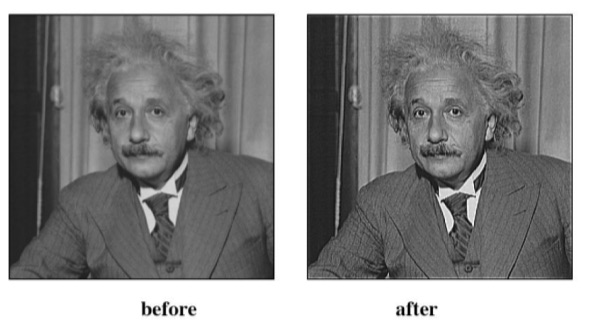
An example of sharpening

Multi-Scale Image Representation

Multi-scale image representation refers to a method that implies having to represent a certain image in various scales.

This is useful since a single template of an object we want to find can be used throughout all the images in the various scales.

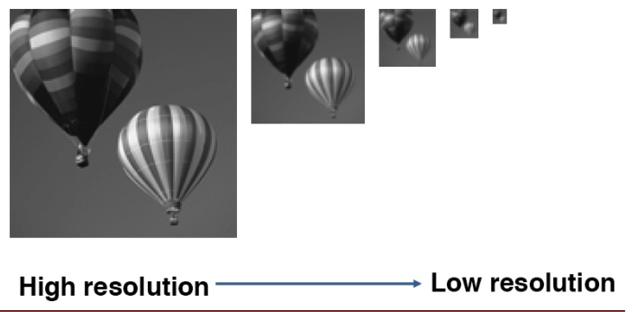
Gaussian Pyramid

In a Gaussian pyramid, the images are obtained by smoothing the original image with the Gaussian filter, and then scaling it down and repeating the process.

It’s essential to smooth the image before downscaling it in order to maintain as much information as possible inside a smaller group of pixels, otherwise, this information would be lost. Subsampling without smoothing will sometimes also lead to aliasing.

It’s computationally convenient to blur the image with a small sigma gaussian filter and then downscale the image by a little scale, for example of 2, and then go on with this procedure.

During a Gaussian pyramid procedure the average of pixels is preserved, but the higher frequencies are lost.

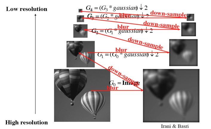
An example of the Gaussian pyramid procedure

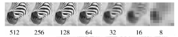
Different edges at different scales represent different information.

For example in the following picture, we can see how in the bigger scale image we ca see the hair on the zebra’s nose; in the smaller images we see the stripes and in the smallest image we only see the animal’s nose.

Edge Detection

Edge detection is a basic operation in image processing since the edges contain much of the important information about the image.

What is an edge

An edge is a more or less sudden change in the intensity of the pixels.

There are 4 types of edges:

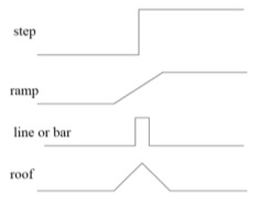
Edge detection based on the 1st derivative

If we take the first derivative of the curve that describes a single line of an image (preferably previously smoothed in order to remove noise), this derivative will have a peak (positive if the intensity increased, negative otherwise) where an edge is.

$$\frac{d}{dx}f(x)=\underset{h\to 0}{\lim }\frac{f(x+h)-f(x)}{h}\approx f(x+1)-f(x)$$

The $h$ in the derivative equation means the increment, since we are dealing with images’ pixels, the increment must be discrete, so we assign it the value of 1.

We can implement this derivative as a linear filter

$$[-1,1]\text{ or }[-1,0,1]$$

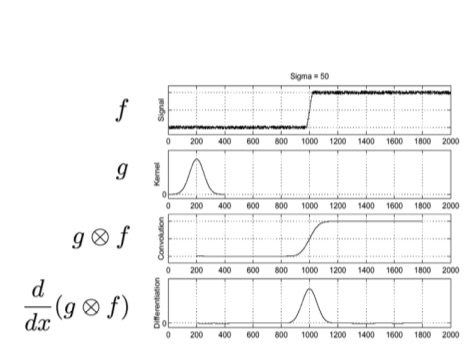
The process of edge detection using the first derivative

Since derivative, as well as convolutions, also linear operations, we can use the associative property to convolute the image with the first derivative of the Gaussian filter.

This is computationally more efficient since the Gaussian kernel, and its derivative, can be pre-calculated, and this would save one operation.

$$\frac{d}{dx}(g\otimes f)=\left(\frac{d}{dx}g\right)\otimes f$$

Thresholding

A threshold is useful to tell the machine how intense a peak should be to be considered an edge.

A second threshold might be used to continue an edge that otherwise would completely stop if using only the first threshold (the edge has a lower magnitude and so it forms a gap).

This technique is called hysteresis and it’s used since in the real world it’s very unusual that an edge completely stops.

2D Edge Detection

Until now we talked about edge detection using derivatives of the curve that describes the intensity of the pixels inside a single line of an image.

If we want to extend the concept to the whole image, we have to calculate two derivatives, one for each direction.

We calculate the derivative in the $x$ direction

$$\frac{d}{dx}I(x,y)=I_x\approx I\otimes D_x$$

And in the $y$ direction

$$\frac{d}{dy}I(x,y)=I_y\approx I\otimes D_y$$

Where

$$\begin{gathered} D_x=\frac{1}{3}\left[\begin{array}{ccccc}-1& & 0& & 1\\ -1& & 0& & 1\\ -1& & 0& & 1\end{array}\right], \\ {D}_y=\frac{1}{3}\left[\begin{array}{ccccc}-1& & -1& & -1\\ 0& & 0& & 0\\ 1& & 1& & 1\end{array}\right] \end{gathered}$$

Edge detection based on the 2nd derivative

It’s also possible to perform edge detection by computing the second derivative of the curve that describes the single line of an image.

In this case, the second derivative would have a “zero crossing” where the edge is located, meaning it would have a low spike and then an high spike, and at the center of it there would be the edge.

This is useful since it betterm marks the intensity of the pixels around the edge.

The kernel to convolve the image in order to obtain this is: $[1,-2,1]$.

Gradient and Magnitude

The gradient is a vector that describes the direction and rate of the fastest increase or decrease of a function $f$ and it’s denoted as $\nabla f$.

$D_x$ is the derivative of $f$ along the $x$ axis, and so only detects changes on the $x$ axis; on the other hand $D_y$ is the partial derivative of $f$ along the $y$ axis, and so only detects the changes on the $y$ axis.

Let $f$ be an image $I$, we can write the gradient in the following way:

$$\nabla I=\left(\frac{\partial I}{\partial x},\frac{\partial I}{\partial y}\right)=(k_x,k_y)$$

Or in general:

$$\nabla f(p)=\left[\begin{array}{c}\frac{\partial f}{\partial x_1}(p)\\ ⋮\\ \frac{\partial f}{\partial x_n}(p)\end{array}\right]$$

The gradient magnitude is a scalar that measures the maximum rate of change. In the image $I$ this can represent how strong an edge is.

The magnitude of $\nabla I$ is

$$\Vert \nabla I\Vert =\sqrt{I_x^2+I_y^2}$$

And the direction of the gradient is given by

$$\theta =arctan(I_y,I_x)$$

Gradient magnitude at different image scales

The scale of the smoothing filter affects the derivative, and so the semantics of the detected edges. Note that strong edges persist across scales.

The gradient magnitude is different at different scales.

Canny edge detector

Canny edge detector is an edge detection operator that proceeds in the following way:

• Smooth the image with a Gaussian filter in order to remove the noise;
• Find the intensity gradient and the direction ($\theta$ slope of the gradient) of the grayscale version of the image by convolving the image with Sobel kernels;
• Apply non-maximum suppression: the image is scanned along the image gradient direction, and if pixels are not part of the local maxima they are set to zero. This has the effect of supressing all image information that is not part of local maxima.
• Apply thresholding in order to remove some remaining edges that may be caused by noise and color variation. We want to remove the lower gradient value edges and keep the higher gradient value edges.
• Track edge by hysteresis;

Laplacian operator

$${\nabla }^{2}f=\frac{{\partial }^{2}f}{\partial x^2}+\frac{{\partial }^{2}f}{\partial y^2}$$

The Laplacian operator is a linear filter that calculates the derivatives over $x$ and $y$ and sums them up.

Since it’s a linear filter, we can convolve it with the Gaussian first and then convole the result with the Image in order to be more efficient.

$${\nabla }^2(G\otimes f)={\nabla }^{2}G\otimes f$$

Laplacian pyramid

The Laplacian pyramid principle is the same as the Gaussian pyramid. They both do some filtering on the image, and then apply the same filtering to the image scaled down.

In this case the Laplacian pyramid is built in the following way:

Let $G_i$ be the image at position $i$ in the Gaussian pyramid, and let $L_i$ be the laplacian of the image $i$.

The Laplacian pyramid is the series of images $L_1,L_2,...,L_n$

We can calculate the Laplacian of the image at position $i$ by taking the difference between $G_i$ and the expanded version of $G_{i+1}$.

$$L_i=G_i-\text{expand}(G_{i+1})$$

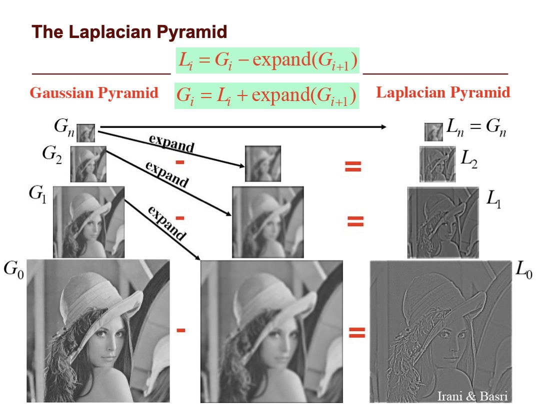
The $L_i$ difference is approximately equivalent to the convolution between the image and laplacian of the Gaussian kernel (${\nabla }^{2}G\otimes f$).

Hough Transformation

Object Identification

The challenges in object identifications are the variations that an objects undergoes when it’s translated into a 2D plane (image).

The factors that changes the image of the 3D object are:

• Viewpoint changes such as:
  • Translation
  • Image-plane rotation
  • Changes of the scale
  • Out-of-plane rotation
• Illumination
• Clutter
• Occlusion
• Noise

Rotation doesn’t remove information from the objects, if the rotation is over the z coordinate (image plane rotation). If we rotate on x or y, (out of plain rotation) we can loose some information, since we see the object in different angles. (We see the back, but we don’t see the front anymore).

In order to do an appearance-based identification or recognition, the objects can be represented by a collection of images, in order to represent the same object under multiple variations. Every instance of this collection is called appearance.

For recognition, a 3D model of the object is not needed, but it’s sufficient to compare the 2D appearances.

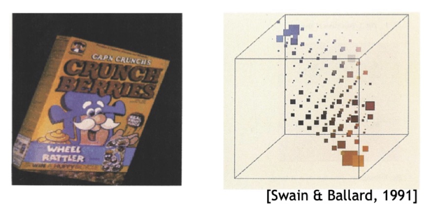
Recognition using color histograms

The idea at the bottom is to represent each appearence with a global descriptor, that will be used to recognize object by matching it with the query image’s descriptor.

Since the colors of an image stays constant under some transformation, we can use it for recognition. The object’s global descriptor will be the color intensity distribution.

The histrogram of color is robust to image translation, but not with out of plain rotation, since the back might be of a different color. This is why we need more pictures.

This recognition method has pros and cons.

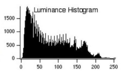
Luminance histogram

The luminance histogram is an histogram which values on the $x$ go from 0 to 255. It describes the distribution of the pixels intensity (from 0 to 255).

The $y$ axis of the histogram tells how many pixels are present of $x$ intensity. It could also be normalized, so the $y$ axis will always be a value betwenn 0 and 1, and it will represent the percentage of the pixels of $x$ intensity inside the whole image.

Color histogram

The luminance histogram is used for grey-value images. In order to use it with colored images, it is necessary to compute an histogram for every channel (Red, Green and Blue). These types of histograms are just like the luminance histograms but tells how many pixels of intensity $x$ and color Red, Green or Blue there are in the image.

3D Joint Color histograms

A 3D Color histogram is represented by a cube of shape $(l,l,l)$ where $l$ is the width of the image.

The cube (three dimensional array) is constructed in a way that in the coordinate $(r,g,b)$ there is number of pixels with that combination of values.

The value of $(r,g,b)$ can be normalized by dividing each component by the sum of the three, in order to have $r+g+b=1$.

3D color histograms are very robust in case of partial occlusion or rotation of the object, unless the oclcusion occlude an entire color of an image that may be distinctive.

RG instead of RGB

Since the Blue component it’s just a linear combination of the Red and Green one ($r+g+b=1$). It’s then possible to only use RG value without loosing information, since $b=1-r-g$.

Histogram Comparison

There are many ways to compare two color histograms.

N.B. All the formulas below refer to normalized histograms.

Intersection

$$\bigcap (Q,V)=\sum _{i}min(q_i,v_i)$$

• It measures the common part of both histograms.
• The result ranges in the interval $[0,1]$,

Euclidean Distance

$$d(Q,V)=\sum _i(q_i-v_i{)}^2$$

• Focuses more on the difference between the histograms.
• The result ranges in the interval $[0,\infty ]$.
• It’s not very discriminant since all the cells are weighted equally.

Chi-square

$${\chi }^2(Q,V)=\sum _i\frac{(q_i-v_i{)}^2}{q_i+v_i}$$

• The result ranges between $[0,\infty ]$
• Cells are not weighted equally: two images with a discriminative color are more similar.

Which measure is the best depends on the application. Both intersection and ${\chi }^2$ are good, the latest being more discriminative. Euclidean is not robust enough.

Nearest-Neighbor strategy

Simple algorithm to get the list of the most similar images of a query image.

1. Build a set of histograms for each view of each know object $H=\{M_1,M_2,M_3,...\}$
2. Build a histogram $T$ for the test image
3. Compare $T$ to each $M_k\in H$ using a suitable comparison measure
4. Select the object with the best matching score, or reject if the distance is above a threshold $t$ (image not similar enough)

Performance Evaluation

Performance evaluation is the process which purpose is to evaluate the system, in order to say that a certain method A is better than another method B.

In this image, we can see the result of the machine-learning algorithm. Every point is the result of an image. The green points are images that contain a positive example, and the blanks are images that contain a negative example.

Let’s say that a positive example is a picture that contains a dog, and a negative one is a picture that doesn’t contain a dog.

The algorithm has to tell us if there is a dog in the image or not.

The more we go toward the top, the more the confidence of the algorithm about the presence of a dog is higher; the more we go to the bottom, the lower the confidence is.

As we can see, the model made some mistakes, since the 3rd image doesn’t contain a dog but the model is quite confident it does.

Threshold

Since the model returns the probability of success, and we need a boolean result, we can set a threshold in order to consider the probability of success or failure.

In this picture, we can see how the results divide in case of a threshold of 0.5.

If the probability outputted by the model is higher than 0.5, we consider the image contains a dog.

Confusion Matrix

A confusion matrix is a table that allows the visualization of the performance of a model.

	Label Positive	Label Negative
Predicted Positive	TP	FP
Predicted Negative	FN	TN

TP, TN, FP, FN

• TP (True Positives): A test result that correctly indicates the presence of a condition or a characteristic (Model: Yes, Ground Truth: Yes)
• TN (True Negatives): A test result that correctly indicates the absence of a condition or a characteristic (Model: No, Ground Truth: No)
• FP (False Positives): A test result that wrongly indicates the presence of a condition or a characteristic. (Model: Yes, Ground Truth: No)
• FN (False Negatives): A test result that wrongly indicates the absence of a condition or a characteristic. (Model: No, Ground Truth: Yes)

Accuracy, Precision, Recall and F1

• Accuracy: $\frac{TN+TP}{N}$ describes how many true predictions the model made out of all the predictions. Describes the rate of correctness, and so also the rate of the wrong predictions.
• Precision: $\frac{TP}{TP+FP}$ describes how good the model is at giving a positive result and actually being right about it. If I raise the threshold, the precision gets higher. This is useful in an emergency situation when I want to do something only if I am very sure about it. I can also apply this if I want to do some heavy calculations only on some occasions, and I want to be sure to do it correctly.
• Recall (True Positive Rate or Sensitivity): $\frac{TP}{TP+FN}$ it describes how many true positives has the model found over all the positives. For example in the case of heart disease patients, a high recall is mandatory since with a low recall the model will not predict heart disease for a patient that actually has it.
• Negative Recall (False Positive Rate or Specificity): $\frac{FP}{TN+FP}=1-\text{Sensitivity}$: it describes how many mistakes the model doing on the positives. For example in an emergency break on an autonomous car, I want this value to be very low otherwise it will be probable that an emergency brake will happen when it’s not necessary.
• F1: $\left(\frac{2}{recal{l}^{-1}+precisio{n}^{-1}}\right)=2\frac{precision\cdot recall}{precision+recall}$. It’s a weighted average of precision and recall. F1 score is usually more useful than just accuracy, especially in uneven class distribution.

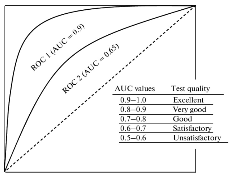
Area under the ROC (Receiver Operator Characteristic) curve (AUC)

The ROC curve is determined by the Recall (True positive rate) and the Negative Recall (False positive rate).

The higher the area under the ROC curve, the better the classifier.

In the case of an area of 0.5, the classifier is just guessing. A perfect classifier should have an AUC of 1, but that’s impossible.

In the case of an area under 0.5, the classifier is worst than guessing, so the solution would be just to invert the result to have a better classifier.

The AUC is useful to set the best threshold since the recall and the other evaluation metrics change depending on the threshold.

Confidence

These types of metrics don’t give any weight to the confidence that a model can have.

For example here the two models, with a threshold $t=50$ have the same values. But the Model B has more confidence since when it says something is successful, it says it with a higher percentage.

Log Loss and Brier Score are two examples of performance evaluation metrics that depend on the confidence of a model.

Linear Regression

Linear regression describes the relationship between two or more variables by fitting a line to the observed data.

We can only use linear regression, which uses a line to fit the data instead of a curve for example for polynomial regression when the relationship between the independent and dependent variables is linear.

Other assumptions are the Homogeneity of variance, the independence of observations, and the normality.

Let’s suppose we have this dataset

Size in feet${}^2$($x$)	Price in 1000$($y$)
2104	460
1416	232
1534	315
852	178

Notation

• $m$ are the number of training examples
• $x^{(i)}$ is the $i^{th}$ feature (input variable)
• $y^{(i)}$ is the $i^{th}$ target variable (output variable)

The hypothesis $h$ is a function that, given an $x$ in input, should output an appropriate $y$. Appropriate in terms of the behavior of the data inside the dataset. In this way, we can estimate the values that are not present in the dataset.

We can write the hypothesis as:

$$h_{\theta }={\theta }_0+{\theta }_{1}x$$

Multivariate linear regression

Let’s assume we have a dataset like this:

Size (feet${}^2$)	Number of bedrooms	Number of floors	Age of home (years)	Price ($1000)
2104	5	1	45	460
1416	3	2	40	232
1534	3	2	30	315
852	2	1	36	178

In this case, we have more than one input variable:

• $m$ is the number of training examples
• $n$ is the number of features
• $x^{(i)}$ is the $i^{th}$ feature (input variable) Example: $x^{(1)}=[5,3,3,2]$.
• $x_j^{(i)}$ is the value of feature $j$ in the $i^{th}$ training example. Example: $x_2^{(1)}=3$.

We can write the hypothesis in the following way:

$$h_{\theta }={\theta }_0+{\theta }_1{x}_1+{\theta }_2{x}_2+...+{\theta }_n{x}_n=\sum _{i=0}^n{\theta }_i{x}_i={\theta }^{T}x$$

For the convention of notation, we define $x_0=1$.

Cost function

Let ${\theta }_i$ be the parameters, how can we choose the right parameters in order to create a line that fits the data?

Let’s assume we’re in a regular linear regression with only one variable. We should choose ${\theta }_0,{\theta }_1$ so that $h_{\theta }(x)$ is the closest to $y$ for the training examples $(x,y)$.

We define the cost function as:

$$J({\theta }_0,{\theta }_1)=\frac{1}{2m}\sum _{i=1}^m(h_{\theta }(x^{(i)})-y^{(i)}{)}^2$$

This function is called the “sum of least squares”, and indicates how much each prediction is close to the real data point.

The goal of linear regression is to minimize $J({\theta }_0,{\theta }_1)$ for the chosen couple ${\theta }_0,{\theta }_1$.

Since $J$ maps every pair of $({\theta }_0,{\theta }_1)$ to a cost, it can be represented in a contour plot.

Or in two dimensions:

In this case, the third dimension is represented by color. So the bluer the line, the lower the cost; the redder the line, the higher the cost.

Measuring Correlation

Two variables are correlated when they track each other. Correlation can be:

• Positive, meaning if one goes up the other goes up too; Example: Person height and shoe size.
• Negative, meaning if one goes up the other goes down. Example: Car weight vs gas mileage.

Causation on the other hand is when a value directly influences another (Education Level → Starting salary). This is almost impossible to find out.

We can measure the level of correlation between two variables with the correlation coefficient (or Pearson coefficient) $r$.

• $r=1$: maximum positive correlation
• $r=0$: no correlation
• $r=-1$: maximum negative correlation

In order to measure correlation without thinking about negative or positive values, we can calculate the $r^2$, which values goes between $0$ and $1$.

The correlation tells us the better the function fits the points, the more corelated $x$ and $y$ are.

Gradient Descent

Gradient descent is an optimization algorithm to find a local minimum of a certain cost function.

The idea is that we have the cost function $J({\theta }_0,{\theta }_1)$. We start with some random values for $({\theta }_0,{\theta }_1)$, and then we keep changing them to progressively reduce $J$.

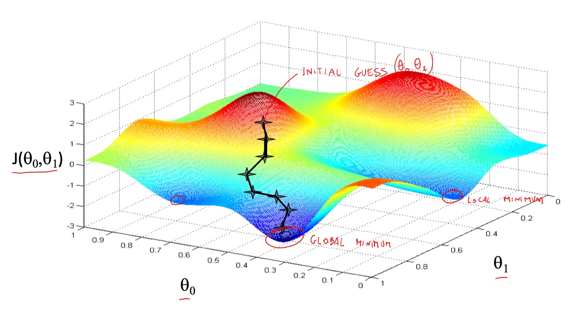
The formal algorithm is the following:

Repeat until convergence

$${\theta }_j:={\theta }_j-\alpha \frac{\partial }{\partial {\theta }_j}J({\theta }_0,{\theta }_1)$$

For $j=0$ and $j=1$ simultaneously. This means that we first calculate both the new values, and only then replace them with the old values. Otherwise, the computing of the second value will be influenced by the already replaced first value.

$\alpha$ is the learning rate, that describes the step size that the algorithm does in order to jump from one cost to another. If $\alpha$ is too small, the gradient descent could take too much time, if it’s too large, it could make the step so big that it overshoots the minimum and diverge.

For the nature of the algorithm, it takes big steps when it’s far from the minimum (slope is higher) and more little steps when it approaches the minimum (slope is lower). This happens because of the slope, and the $\alpha$ doesn’t change.

The algorithm stops (the convergence is declared) when the step size is very small (such as 0.001) or when it has done a certain number of iterations.

Application to the Linear Regression

Since the cost function $J({\theta }_0,{\theta }_1)$ in the case of linear regression is defined as seen, we have to calculate its derivative with respect to every ${\theta }_j$.

$$\begin{gathered} j=0:\frac{\partial }{\partial {\theta }_0}J({\theta }_0,{\theta }_1)=\frac{1}{m}\sum _{i=1}^m(h_{\theta }(x^{(i)})-y^{(i)})\cdot 1 \\ j=1:\frac{\partial }{\partial {\theta }_1}J({\theta }_0,{\theta }_1)=\frac{1}{m}\sum _{i=1}^m(h_{\theta }(x^{(i)})-y^{(i)})\cdot x^{(i)} \end{gathered}$$

Polynomial Regression

In some cases, there is not a linear relationship between the features, meaning that, in the case of two features, they cannot be modeled by a line.

An example is how the price of a house changes. It may change a lot in case the size is small, but the change in price can become less and less significant to the change in the size when this value becomes bigger.

So we don’t only consider the value of a feature, but we also the squared, the square root, or the cube of it, depending on how the value may change.

Let $x$ and $y$ repectively be the size and the price of an house. An example of an hypotesis for the polynomial regression could be

$$h_{\theta }(x)={\theta }_0+{\theta }_{1}x+{\theta }_2{x}^2+{\theta }_3{x}^3$$

In case $x\in [1,1000]$ , then $x^2\in [1;10\cdot 10^6]$ and $x^3\in [1;10\cdot 10^9]$ .

Since the features can have values that are very different from each other, and so the gradient descent will take a long time to execute, it’s necessary to normalize the features.

Normal Equation

The normal equation is a way to minimize $J(\theta )$ in an analytical way, meaning there is no need to iterate an algorithm.

The gradient of a function $f(p)$ is an array of dimension $n$ where $n$ is the number of variables inside the function $f(p).$ The array contains the partial derivative of $f$ with respect to every possible variable.

$$\nabla f(p)=\left[\begin{array}{c}\frac{\partial f}{\partial x_1}(p)\\ ...\\ \frac{\partial f}{\partial x_n}(p)\end{array}\right]\in {\mathbb{R}}^n$$

Since the gradient descent calculates the new theta according to this equation

$$\theta :=\theta -\alpha {\nabla }_{\theta }J$$

We can solve the gradient of $J$ with respect to $\theta$ analytically.

$${\nabla }_{\theta }J=\left[\begin{array}{c}\frac{\delta J}{\delta {\theta }_0}(p)\\ ...\\ \frac{\delta J}{\delta {\theta }_n}(p)\end{array}\right]\in {\mathbb{R}}^{n+1}$$

Let $A$ be a matrix of $n\text{ x }m$, and the function $f(A)\in \mathbb{R}$ we can calculate the gradient of $f$ with respect to $A$:

$${\nabla }_{A}f(A)=\left[\begin{array}{ccccc}\frac{\delta f}{\delta A_{11}}& & \dots & & \frac{\delta f}{\delta A_{1n}}\\ ⋮& & \ddots & & ⋮\\ \frac{\delta f}{\delta A_{m1}}& & \dots & & \frac{\delta f}{\delta A_{mn}}\end{array}\right]$$

Trace

We define the trace of a square matrix as the sum of the elements on its main diagonal.

$$trA=\sum _{i=1}^n{A}_{ii}$$

Some properties of matrix derivatives:

1. $trAB=trBA$
2. $trABC=trCAB=trBCA$
3. $f(A)=trBA\in \mathbb{R}$ where ${\nabla }_{A}trAB=B^T$
4. $trA=tr{A}^T$
5. If $a\in \mathbb{R}\to \text{tr }a=a$
6. ${\nabla }_{a}trAB{A}^{T}C=CAB+C^{T}A{B}^T$

CONTINUE THIS THING (You can see the continuation on the stanford lecture notes)

Locally Weighted Regression

💡 Difference between parametric and non parametric models: - **Parametric** models are those that require the specification of some paremeters in order to make a prediction. For example in linear regression we have the $\theta$'s. - **Non-parametric** models di not rely on specific parameters (examples are SVMs, KNNs or Histograms) and therefore often produce more accurate results.

In the classic linear or polynomial regression, all the samples have the same weight.

In case of locally weightet regression, we assume that the set of data between the new data I want to test it’s more related to it than the further data, so the model weights it more.

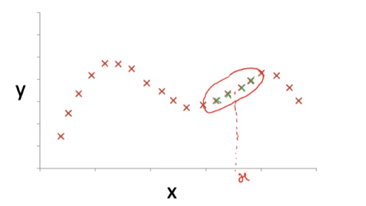
We calculate the weight

$$w^{(i)}=\exp \left(\frac{-\Vert x^{(i)}-x\Vert }{2{\tau }^2}\right)$$

If $\Vert x^{(i)}-x\Vert$ is small, the weight approaches 1, it approaches 0 if $\Vert x^{(i)}-x\Vert$ is large.

$\tau$ (Tau) is an hyperparameter and represents the bandwidth.

The $x$ in the weight equation is the new $x$ we want to test, so the weight is computed at test time.

With this type of regression, the aim is to fit $\theta$ to minimize

$$\sum _{i=1}^m{w}^{(i)}(y^{(i)}-{\theta }^T{x}^{(i)}{)}^2$$

Likelihood

When we calculate the $y$’s, we assume there is some kind of error $ϵ$.

Here’s the equation for linear regression:

$$y^{(i)}={\theta }^T{x}^{(i)}+{ϵ}^{(i)}$$

This error may be caused by the random noise in the sensor or by the unmodelled effects, since we surely will make some errors in modelling the world in some way.

We also assume that the error is distributed according to a gaussian with $0$ mean and a standard deviation of ${\sigma }^2$.

We choose the gaussian since it’s simple and since a lot of errors are gaussians. Another important fact that made us choose this kind of distribution over the other is the central limit theorem, that says if you have a sufficently large population and you take many random saples from this population (with replacement), then the distribution of the samples will be approximately gaussian.

$${ϵ}^{(i)}\sim N(0,{\sigma }^2)$$

We can also write the probability of the error as

$$P({ϵ}^{(i)})=\frac{1}{\sqrt{2\pi }\sigma }exp\left(\frac{-({ϵ}^{(i)}{)}^2)}{2{\sigma }^2}\right)$$

We can also calculate the probability of $y^{(i)}$ given $x^{(i)}$ parametrized by $\theta$

$$P(y^{(i)}|x^{(i)};\theta )=\frac{1}{\sqrt{2\pi }\sigma }exp\left(-\frac{(y^{(i)}-{\theta }^T{x}^{(i)}{)}^2}{2{\sigma }^2}\right)$$

We assume that ${\theta }^T{x}^{(i)}$ is the mean, so

$$y^{(i)}|x^{(i)};\theta \sim N({\theta }^T{x}^{(i)},{\sigma }^2)$$

We can define the likelihood as

$$L(\theta )=P(\overrightarrow{y}|X;\theta )=\prod _{i=1}^{m}P(y^{(i)}|x^{(i)};\theta )$$

And the log likelihood as

$$\ell (\theta )=\log L(\theta )$$

From this equation, we obtain

$$\ell (\theta )=m\log \frac{1}{\sqrt{2\pi }\sigma }+\sum _{i=1}^m-\frac{(y^{(i)}-{\theta }^T{x}^{(i)}{)}^2}{2{\sigma }^2}$$

If I take the maximum likelihood estimation (MLE), I’m choosing $\theta$ in order to maximise $L(\theta )$ and so also $\ell (\theta ).$ Is possible to subsitute the Likelihood with it’s logarithm since the logarithm is a monotonous function (if $x$ increases, also $y$ increases), and so it ensures that the maximum value of the log of the probability occurs at the same point as the original probability function.

This is equal to minimizing the second term (I don’t consider the first term since it doesn’t depend on theta). The second term is just the cost function $J(\theta )$.

In other words, the MLE state that we can maximise the Likelihood by minimizing the log likelihood. To do this we just have to calculate the derivative of the likelihood find the zeros. We can do it analytically or with techniques like gradient descent.

Logistic Regression

Logistic regression is different from linear regression since it’s used for classification. Classification means that there are $n$ classes of objects, so $y\in \{0,1,2,..,n\}$ and the model gives out a probability that the object belongs to one of these classes

Classification with 2 classes

The simplest classification is when there are only two classes. In this case $y\in \{0,1\}$. In general 0 is the negative class and 1 is the positive one.

We will have a function $h_{\theta }(x)$ that gives us the probability of the object being in one of the two classes. We have to set a threshold, but assuming the threshold is 0.5, we’ll have:

• Predict $y=1$ if $h_{\theta }(x)\ge 5$;

• Prediuct $y=0$ otherwise.

• Example

  Let’s say we have a model that predict the sentiment of a phrase based on how many times the words “awful” and “awesome” appear. The number of times the words appear are the features.

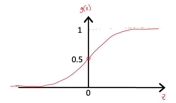
In linear regression $h_{\theta }(x)$ can be greater than 1 and smaller than 0, we can’t use it to model a probabiliy. In order to “squash” the function between 0 and 1, we can use the sigmoid function (also called logistic function).

$h_{\theta }(x)$ remains equal to ${\theta }^{T}x$ but we apply the sigmoid in order to squash it in the 0,1 interval.

$$h_{\theta }(x)=g({\theta }^{T}x)$$

Where

$$g(z)=\frac{1}{1+e^{-z}}$$

The interpretation of the hypotesis ($h_{\theta }(x)$) output is that it describes the probability that $y=1$ on the input $x$. So if $h_{\theta }(x)=0.7$ there’s a $70\%$ probability that $x$, parametrized by $\theta$ is in class 1:

$$h_{\theta }(x)=P(y=1|x;\theta )$$

Since in this case there are only two classes, we have that:

$$P(y=0|x;\theta )+P(y=1|x;\theta )=1$$

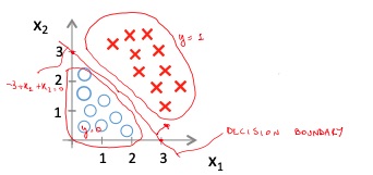
Linear decision boundaries

If $g(z)\ge 0.5$, then $z\ge 0$ and $y=1$

If $g(z)<0.5$, then $z<0$ and $y=0$

So the decision boundary happens when $z$ changes sign

Let’s assume we have more than just a feature, and let’s assume the function is

$$h_{\theta }(x)=g({\theta }_0+{\theta }_1{x}_1+{\theta }_2{x}_2)$$

Then, applying what we said before, we can predict $y=1$ if ${\theta }^{T}x=-3+x_1+x_2\ge 0$, where this equation is the equation of the line that represent the decision boundary.

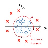
Non-linear decision boundaries

We can also have a decision boundary that’s not a line, but some type of curve. The curve could also be a circle, inside of which there are all the samples belonging to a class and outside the rest of the samples.

Learn $\theta$s with logistic regression

Since we know that $h_{\theta }(x)=P(y=1|x;\theta )$, we can generalize the formula as:

$$P(y|x;\theta )=h_{\theta }(x{)}^y(1-h_{\theta }(x){)}^{1-y}$$

We also can define the Log Likelihood in the case of Logistic Regression as:

$$\begin{gathered} L(\theta )=P(\overrightarrow{y}|X;\theta )=\prod _{i=1}^{m}P(y^{(i)}|x^{(i)};\theta ) \\ =\prod _{i=1}^m{h}_{\theta }(x^{(i)}{)}^{y^{(i)}}(1-h_{\theta }(x^{(i)}){)}^{1-y^{(i)}} \end{gathered}$$

and the log likelihood as:

$$\ell (\theta )=\sum _{i=1}^m{y}^{(i)}\log (h_{\theta }(x^{(i)}))+(1-y^{(i)})\log (1-h_{\theta }(x^{(i)}))$$

The gradient ascent algorithm updates the theta vector with the following rule:

$${\theta }_j:={\theta }_j+\alpha \frac{\partial }{\partial {\theta }_j}\ell (\theta )$$

Where

$$\frac{\partial }{\partial {\theta }_j}\ell (\theta )=\sum _{i=1}^m\left(y^{(i)}-h_{\theta }(x^{(i)})\right)x_j^{(i)}$$

Newton’s Method for Optimization

The Newton’s method for optimization is another iterative method that allows to find $\theta$ such that $f(\theta )=0$ where $f$ is a given function. This method is another iterative optimization method that can be used as an alternative to the gradient descent method.

This method tells us that we can update the $\theta$ with the following rule:

$${\theta }^{(t+1)}:={\theta }^{(t)}-\frac{{\ell }^{\prime }({\theta }^{(t)})}{{\ell }^{\prime \prime }({\theta }^{(t)})}$$

Where ${\ell }^{\prime \prime }(\theta )$ is the second derivative of the log likelihood.

Derivative, Jacobian and Hessian difference on Stack Exchange

The pro of this method is that there isn’t any hyperparameter, but the method requires an higher order of differentiability for the loss function.

Case for when $\theta$ is a vector

In the general case, when $\theta$ is a vector, we can use the following update rule:

$${\theta }^{(t+1)}:={\theta }^{(t)}-H^{-1}{\nabla }_{\theta }\ell$$

Where $H$ is the hessian matrix defined as $H_{ij}=\frac{{\partial }^2\ell }{\partial {\theta }_i\partial {\theta }_j}$.

Exponential Family of Distributions

Wikipedia page for Exponential Family of Distribution

The exponential family is a set of distributions whose probability distribution can be described by a general equation:

$$P(y|\eta )=b(y)\exp \left({\eta }^{T}T(y)-a(\eta )\right)$$

Where:

• $\eta$ is the natural parameter
• $T(y)$ is the succifient statistic
• $b(y)$ is the base measure (scalar)
• $a(\eta )$ is the log-partition function
• $y$ is the data (scalar)

$\eta$ and $T(y)$ can be scalars or vectors, but their shape must match.

Example with the Bernoulli Distribution

We know that if $y$ is a random variable that distributes according to a Bernoulli Distribution $y\sim Ber(\varphi )$, that

$$\begin{gathered} P(y;\varphi )={\varphi }^y(1-\varphi {)}^{1-y} \\ =\exp \left(\log {\varphi }^y(1-\varphi {)}^{1-y}\right) \\ =\exp \left(y\log \varphi +(1-y)\log (1-\varphi )\right) \\ =\exp \left(\log (\frac{\varphi }{1-\varphi })y+\log (1-\varphi )\right) \end{gathered}$$

We can see how the final formula can be mapped to the general family of distribution equation:

• $\eta =\log (\frac{\varphi }{1-\varphi })$
• $T(y)=y$
• $-a(\eta )=\log (1-\varphi )$
• $b(y)=1$

Generalized Linear Models

Before all let’s make some assumptions, that are design choises:

1. $y|x;\theta \sim \text{ExpFamily}(\eta )$;
2. Given $x$, we want to have $h_{\theta }(x)=E[T(y)|x]$;
3. $\eta ={\theta }^{T}x$. If $\eta$ is a vector, then ${\eta }_i={\theta }_i^{T}x$, meaning that the parameter $\eta$ and the input are linearly related.

GLM for Ordinary Least Squares

We can see that Ordinary Least Squares is a special case of GLM family of models, since we have:

$$\begin{array}{rlr}{h}_{\theta }(x)=E[T(y)|x]& & \text{(Assumption 2)}\\ =\mu & & (\text{because }y|x;\theta \sim \mathcal{N}(\mu ,{\sigma }^2))\\ =\eta & & \\ ={\theta }^{T}x& & \text{(Assumption 3)}\end{array}$$

Multinomial Classification

Multinomial classifications is more or less the same problem of classification but with more than two classes.

When we were dealing with two classes classifications, we were using logistic regression. Now this is not the case anymore, and we need more advanced methods.

Softmax Function

The softmax function is the extension of the sigmoid function when we have more than two classes.

The softmax function applied to the index $i$, computes the probability of the object of being in the $i$-th class.

$$P_i=\frac{e^{x_i}}{{\sum }_{j=1}^K{e}^{x_j}}$$

We can prove that the softmax function is the response function derived by the link function that connects softmax regression to the exponential family of distribution.

• Proof that the softmax regression is part of the exponential family of distribution

  To parametrize a multinomial over $k$ possible outcomes ($k=3$ for example if we want to classify an email in spam, personal and work) we can use $k-1$ parameters ${\varphi }_1,...,{\varphi }_{k-1}$ since the last parameter ${\varphi }_k$ is just a combination of the previous ones (because they have to satisfy the property $\sum {\varphi }_i=1$).

  We can express the multinomial as an exponential family distribution. We first have to define the concept of a “one-hot” vector, which is a vector $T(y)$ in which the $y$-th element has value $1$ and all the other elements have value 0.

  In the case of softmax regression, we’ll have $T(y)\in {\mathbb{R}}^{k-1}$ where $T(y{)}_i=1\{y=i\}$.

  We also have that $\mathcal{E}[T(y{)}_i]=P(y=i)={\varphi }_i$.

  Starting from that, we can see how the multinomial it’s a member of the exponential family, by mapping the $\eta$’s to the $\varphi$’s through the softmax function.

  $$\begin{array}{rl}p(y;\varphi )=& {\varphi }_1^{1\{y=1\}}{\varphi }_2^{1\{y=2\}}\cdots {\varphi }_k^{1\{y=k\}}\\ =& {\varphi }_1^{1\{y=1\}}{\varphi }_2^{1\{y=2\}}\cdots {\varphi }_k^{1-{\sum }_{i=1}^{k-1}1\{y=i\}}\\ =& {\varphi }_1^{(T(y){)}_1}{\varphi }_2^{(T(y){)}_2}\cdots {\varphi }_k^{1-{\sum }_{i=1}^{k-1}(T(y){)}_i}\\ =& \exp ((T(y){)}_1\log \left({\varphi }_1\right)+(T(y){)}_2\log \left({\varphi }_2\right)+\\ & \cdots +\left(1-\sum _{i=1}^{k-1}(T(y){)}_i\right)\log \left({\varphi }_k\right))\\ =& \exp ((T(y){)}_1\log \left({\varphi }_1/{\varphi }_k\right)+(T(y){)}_2\log \left({\varphi }_2/{\varphi }_k\right)+\\ & \cdots +(T(y){)}_{k-1}\log \left({\varphi }_{k-1}/{\varphi }_k\right)+\log \left({\varphi }_k\right))\\ =& b(y)\exp \left({\eta }^{T}T(y)-a(\eta )\right)\end{array}$$

  Where the exponential family parameters are mapped to the multinomial logistic regression as following:

  $$\begin{array}{rl}\eta & =\left[\begin{array}{c}\log \left({\varphi }_1/{\varphi }_k\right)\\ \log \left({\varphi }_2/{\varphi }_k\right)\\ ⋮\\ \log \left({\varphi }_{k-1}/{\varphi }_k\right)\end{array}\right]\\ a(\eta )& =-\log \left({\varphi }_k\right)\\ b(y)& =1.\end{array}$$

  And ${\eta }_i=\log \frac{{\varphi }_i}{{\varphi }_k}$ is the link function. In order for the link function to be invertible, we set ${\eta }_k=0$, so we have:

  $$\begin{array}{rl}{e}^{{\eta }_i}& =\frac{{\varphi }_i}{{\varphi }_k}\\ {\varphi }_k{e}^{{\eta }_i}& ={\varphi }_i\\ {\varphi }_k\sum _{i=1}^k{e}^{{\eta }_i}& =\sum _{i=1}^k{\varphi }_i=1\end{array}$$

  This implies that ${\varphi }_k=1/{\sum }_{i=1}^k{e}^{{\eta }_i}$, and so we have that:

  $${\varphi }_i=\frac{e^{{\eta }_i}}{{\sum }_{j=1}^k{e}^{{\eta }_j}}$$

  This is the response function, and it’s the softmax function.

Softmax Regression (multinomial logistic regression)

The softmax regression model’s hypothesis will take an example $x$ in input and will output the following:

$$\begin{array}{rl}{h}_{\theta }(x)& =\mathrm{E}[T(y)\mid x;\theta ]\\ & =\mathrm{E}\left[\begin{array}{c}1\{y=1\}\\ 1\{y=2\}\\ ⋮\\ 1\{y=k-1\}\end{array}\right]x;\theta ]\\ & =\left[\begin{array}{c}{\varphi }_1\\ {\varphi }_2\\ ⋮\\ {\varphi }_{k-1}\end{array}\right]\\ & =\left[\begin{array}{c}\frac{\exp \left({\theta }_1^{T}x\right)}{{\sum }_{j=1}^k\exp \left({\theta }_j^{T}x\right)}\\ \frac{\exp \left({\theta }_2^{T}x\right)}{{\sum }_{j=1}^k\exp \left({\theta }_j^{T}x\right)}\\ ⋮\\ \frac{\exp \left({\theta }_{k-1}^{T}x\right)}{{\sum }_{j=1}^k\exp \left({\theta }_j^{T}x\right)}\end{array}\right].\end{array}$$

Meaning if we apply the softmax regression to a vector $x$ of parameters, we’d have a vector of size $N\text{x}K$ where $N$ is the number of samples and $K$ is the number of classes, that tells us the probability distribution of every sample, formally the probability $p(y=i|x;\theta )$ for every $i=1,...,k$.

Learn $\theta$s with Softmax Regression

If we have a training set of $n$ examples $\{(x^{(i)},y^{(i)}{\}}_{i=1}^n$ and would like to learn the ${\theta }_i$ parameters of the model, we begin by writing the log-likelihood

$$\begin{array}{rl}\ell (\theta )& =\sum _{i=1}^n\log P\left(y^{(i)}\mid x^{(i)};\theta \right)\\ & =\sum _{i=1}^n\log \prod _{l=1}^k{\left(\frac{e^{{\theta }_l^T{x}^{(i)}}}{{\sum }_{j=1}^k{e}^{{\theta }_j^T{x}^{(i)}}}\right)}^{1\left\{y^{(i)}=l\right\}}\end{array}$$

We can then obtain the Maximum Likelihood Estimate by mamixising $\ell (\theta )$ using gradient ascent or Newton’s method.

Image Classifications with Linear Classifiers

Image classification is the act of labeling an image with a certain class. The problem is that the computer elaborates images as a grid of RGB values, that changes dramatically in case of camera movement, environment illumination and other things.

Other problems that can prevent the computer to recognize the object are background clutter, deformation of the object, occlusion and intraclass variation.

Since it doesn’t exists a precise algorithm that can get an image as input and tell if there is a certain object in it or not, the idea is to collect a dataset of image and labels, use machine learning to train a classifier and predict the new images using the trained classifier.

Nearest Neighbor Classifier

This classifier uses the L1 (Manhattan) distance, defined as $d_1(I_1,I_2)={\sum }_p|I_1^p-I_2^p|$, in order to find the most similar image to a given one.

Let $N$ be the examples, the training has complexity $O(1)$ and the prediction has complexity $O(N)$.

This because in the training part, the classifier just memorize the training data.

In the prediction part, the classifier analyzes every train image and predicts the label of the nearest image.

This isn’t optimal since we prefer a classifier that has a slow training but a fast prediciton.

K-Nearest Neighbors

K-Nearest neigtbors is an optimization of the nearest neighbor classifier, in which only a subset of $K$ closest points is chosen, insted of the entire set of points. In this way the algorithm is more efficient, even if the solution would be less precise.

This method uses also another type of distance, that’s the Euclidean distance $d_1(I_1,I_2)=\sqrt{{\sum }_p(I_1^p-I_2^p{)}^2}$.

This method is never used on images since it’s very slow at test time, and distance metrics on pixels are not inforamtive.

Linear Classification

A linear classifier is a classifier that makes the decision upon a linear combination of the data given in input.

This data $x$ is combined with a weight $W$ and some biases $b$. So the function can be written as $f(x,W)=Wx+b$. The output is a vector of $k$ dimension, where $k$ is the number of classes, that describes the probability distribution of the image to belong in that class.

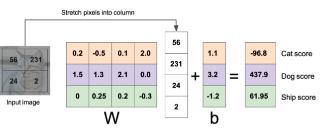
Example with an image of 4 pixels and 3 classes

Loss Functions and Optimization

In order to quantify whether we have choosen a good or bad values for $W$, we can initialize those value at random, define a loss function, and find a $W$ that minimizes that function.

Given a dataset of examples $\{(x_i,y_i){\}}_{i=1}^N$ where $x_i$ is the image and $y_i$ is an integer label, we can define the loss function as

$$L=\frac{1}{N}\sum _i{L}_i(f(x_i,W),y_i)$$

When using a linear classifier, the output is an array of unnormalized log-probabilities. We can use the softmax function to trasnform these values in normalized probability, in order to interpret the array as a probability distribution.

We can choose the weights to maximise the likelihood of the probabilities. So we can define

$$L_i=-\log P(Y=y_i|x=x_i)=-\log \frac{e^{x_k}}{{\sum }_j{e}^{x_j}}$$

Regularization

Regularization prevents the model from overfitting (doing too well on training data), because that would cause bad performance when working with new data. This is done by adding a factor $\lambda R(W)$ at the end of the loss function $L(W)$.

• $\lambda$ is the regularization strenght, and it’s a hyperparameter.
• $R(W)$ can vary:
  • L2 regularization: $R(W)={\sum }_k{\sum }_l{W}_{k,l}^2$
  • L1 regularization: $R(W)={\sum }_k{\sum }_l|W_{k,l}|$
  • Elastic net (L1 + L2): $R(W)={\sum }_k{\sum }_l\beta W_{k,l}^2+|W_{k,l}|$

Optimization

Gradient Check

Computing the gradient of an array of values in the numerical way, meaning applying the definition of derivative $\frac{f(W)}{dW}={\lim }_{h\to 0}\frac{f(W+h)-f(W)}{h}$ with a small value for $h$, is not very optimal, since there is a lot of computation going on, and the result is only an estimation.

Gradient check is a technique used to check the correctness of the implementation of the backpropagation algorithm in a neural network. It involves comparing the analytically computed gradients of the model’s parameters with the gradients computed using finite differences. If the two values are close, it indicates that the implementation is correct. It is a useful tool for debugging and can help detect errors such as mistakes in the computation of the gradients or bugs in the code.

Image Features

In images, we can take the raw pixels as our features. This can be a great decision for simple problems, since it doesn’t require to modify the data we have in some other ways; but for neural networks it’s not enough.

If we compute some other data from the image beforehad, we may achieve better performance. For example color histograms could be a good idea for some problems.

Let’s assume we have some points, some belonging to a class, some to the other, distributed in a circle around the origin. We cannot separate the two classes with a linear classifier, but if we change the data and map every point to the distance it has from the origin, then we may have some data that’s easier to work with, and it’s now possible to separate the classes with a linear classifier.

A more recent technique is to to compute the Hisogram of Oriented Gradients, meaning to consider the derivative of all patches of the images (small sections). A patch with a brighter color towards a directions means that there is a strong edgeness on that direction. This performance better than the color histogram.

We may also combine different features togheter to have a stronger representation.

What deep neural networks do is extract features from an image in some smart way, instead of extracting features with a design method.

Backpropagation

Backpropagation is an efficient and accurate way to compute the gradient of a loss funcion.

The process happens in two phases:

1. Forward pass: we compute the outputs of every node and calculate the final loss of the network according to a certain loss function.
2. Backward pass: starting from the end of the network, we recursively apply the chain rule to compute the gradients all the way to the inputs of the network. The gradient is used then to update the weights.

Example

(Source)

Let’s assume the loss function is

$$f(a,b,c)=(a+b)(b+c)$$

Let’s assume that $a=-1,b=3,c=4$

In order to easily analyze expression, we can also draw the computational graph of the loss function

Every node ($x$, $y$ and $f$) in the computational graph can compute two things without being aware of the rest of the graph:

• Output of the node
• Local gradient of the node

Output	Local gradients
$x=a+b$	$\frac{\partial x}{\partial a}=1,\frac{\partial x}{\partial b}=1$
$y=b+c$	$\frac{\partial y}{\partial b}=1,\frac{\partial y}{\partial c}=1$
$f=x\cdot y$	$\frac{\partial f}{\partial x}=y,\frac{\partial f}{\partial y}=x$

Remember that the chain rule state that:

$$\frac{\partial f}{\partial y}=\frac{\partial f}{\partial q}\frac{\partial q}{\partial y}$$

We define the upstream gradient as the gradient calculated in the forward phase that’s now backpropagating. Each step in the backpropagation, we calculate the new gradient to backpropagate as the product of the local gradient and the upstream gradient.

Example of the backpropagation process using the recursive appllication of the chain rule with the local and upstream gradient.

Backpropagation with vectors and matrices (or tensors)

If we are dealing with vectors, matrices or tensors, then the process is the same but we’re not longer calculating regular derivatives. Of course the computational power needed to compute the gradients or jacobians is much more than the regular derivatives.

Vector Derivatives Recap

• If $x\in \mathbb{R},y\in \mathbb{R}$, then we have the regular derivative $\frac{\partial y}{\partial x}\in \mathbb{R}$ that tells us how much will $y$ change if $x$ changes by a small amount;
• If $x\in {\mathbb{R}}^N,y\in \mathbb{R}$, then the derivative is the Gradient $\frac{\partial y}{\partial x}\in {\mathbb{R}}^N$ where $(\frac{\partial y}{\partial x}{)}_n=\frac{\partial y}{\partial x_n}$. This tells us, for each element $x_i\in x$, how much will $y$ change if $x_i$ changes by a small amount.
• If $x\in {\mathbb{R}}^N,y\in {\mathbb{R}}^N$, then the derivative is the Jacobian $\frac{\partial y}{\partial x}\in {\mathbb{R}}^{N\times M}$ where $(\frac{\partial y}{\partial x}{)}_{n,m}=\frac{\partial y_m}{\partial x_n}$. This tells us for each element $x_i\in x$, how much will every element $y_i\in y$ change if $x_i$ changes by a small amount.

Convolutional Neural Networks

Convolutional neural networks are neural networks that use kernel convolution in order to predict something.

Those types of NN are mostly used for image classification.

Image Classification with CNN

This because having the entire image, meaning a vector made up with all the image’s pixels, as the input parameters for a NN is not possible under a computational point of view, since there would be too many nodes and connections.

CNN’s also take the full image as the input, but they do some operations, specifically some kernel convolutions, in order to learn which are the most discriminant filters that are able to improve the performances.

In a CNN, there are three types of layers.

Convolution Layer

In this layer, the image is convolved with a kernel that has smaller dimensions but the same depth. In case of RGB image the depth is 3 because it includes the RGB color channels.

The convolution generates a smaller image that’s called activation map.

Every filter generates a different activation map of the same dimension. At the end of this layer we’ll have an image of increased depth (the number of activation maps) but smaller size.

Activation Layer

In the activation layer, the activation map is given as an input to a certain activation function, such as ReLu, SoftMax or SoftPlus. This is needed in order to insert some non-linearity, otherwise the model coudn’t be able to learn more complex patterns.

Pooling Layer

Pooling is an operation that takes a patch from the image and gives some kind of output that’s smaller than the original image.

Pooling is useful to reduce the image resolution. We can use a bigger slide in the convolution as an alternative.

We distinct between two types of pooling:

• Max Pooling: given a patch of $k\text{ x }k$ filter and a slide such that the filters don’t overlap, it outputs an image that’s $k$ times smaller, and each patch it’s mapped with its maximum value.
• Average Pooling: Is the same as max pooling, but instead of taking the maximum value from each patch, it takes the average value.

---

After some stages of repeatingly applying convolution, activation and pooling, we reach the final layer, that’s a classic fully connected layer as in an ordinary Neural Network. This layer takes as input the last output given by the last pooling layer, and ouputs the probability of the image being in a certain class.

In the first layer, we’ll have the filters that the network has computed, deeper we go, more abstract the images would be.

The important thing of CNN is that the model learns the most important features and what the image represent at the same time. We can use backpropagation in order to optimize the weights and biases.

Generative Learning Algorithms

Standford Lecture Source

Generative Learning Algorithms differ from the Discriminant Learning Algorithms that we’ve seen so far (Linear and Logistic regression for example) because they look at each class of elements in an isolated way.

A discriminative learning algorithm learns $P(y|x)$ where the $x$ is the feature and $y$ is the class.

A generative learning algorithm learns $P(x|y)$. This types of algorithms also learn $P(y)$, that’s called class prior. This is useful to know the probability distribution of the classes, before having seen the features.

Using Bayes rule, when a new example comes in, it’s possible to calculate the $P(y|x)$:

$$P(y=1|x)=\frac{P(x|y=1)P(y=1)}{P(x)}$$

Where

$$P(x)=P(x|y=1)P(y=1)+P(x|y=0)P(y=0)$$

GDA - Gaussian Discriminant Analysis

Let’s suppose that $x\in {\mathbb{R}}^n$, so we drop the $x_0=1$ convention.

Let’s assume that $P(x|y)$ is distributed as a Gaussian.

GDA, instead of fitting a line that separates the two classes like in Logistic Regression, fits two multivariate gaussians, one for each classes. The seprataion of the examples with two gaussians implies a decision boundary that’s very similar to the line fitted by the Logistic Regression.

Multivariate Gaussian

In a multivariate gaussian $Z\sim N(\vec{\mu },\Sigma )$ the elements on the covariance matrix $\Sigma$’s diagonal determines the height and base of the bell, meanwhile the other elements determines its orientation.

Note that every covariance matrix is symmetric.

Changing the values in the $\mu$ vector, changes the position of the center of the gaussian around the plain.

Note that:

$$P(Z)=\frac{1}{2{\pi }^{\frac{n}{2}}|\Sigma {|}^{\frac{1}{2}}}\exp \left(-\frac{1}{2}(z-\mu {)}^T{\Sigma }^{-1}(z-\mu )\right)$$

GDA is parametrized by ${\mu }_0\in {\mathbb{R}}^n,{\mu }_1\in {\mathbb{R}}^n,\Sigma \in {\mathbb{R}}^{n\times n},\varphi \in \mathbb{R}$

Where ${\mu }_0,{\mu }_1$ are the means for the class 0 and class 1, and $\varphi =P(y=1)$ because $P(y)$ is distributed as a Bernoulli.

💡 GDA is a generalized term to describe both LDA and QDA. They're very similar, with the only difference that LDA has only one shared covariance matrix for every class, and QDA provides a different covariance matrix for each and every class. Most of the time we’ll use two different means but only one covariance matrix because most of the problems in which GDA (LDA in particular) is applied are about finding a linear boundary. In case we’d use two covariance matrixes (QDA), the boundary would be not linear anymore, but this is not so useful since the result will be similar, but having twice the number of parameters increases the computational power needed.

In Generative learning algorithms, we want to maximise the joint likelihood defined as:

$$\begin{gathered} L(\varphi ,{\mu }_0,{\mu }_1,\Sigma )=\prod _{i-1}^{n}P(x^{(i)},y^{(i)};\varphi ,{\mu }_0,{\mu }_1,\Sigma )= \\ \prod _{i-1}^{n}P(x^{(i)}|y^{(i)})P(y^{(i)}) \end{gathered}$$

Note

This is different from the Discriminant learning algorithms, where we wanted to maximize the conditional likelihood defined as:

L(\theta) = \prod_{i=1}^nP(y^{(i)}|x^{(i)};\theta)

The difference is that in the discriminant learning algorithms we want to find parameters that maximise the probability of $y$ given $x$, meanwhile in the Generative learning algorithms we want to find parameters that maximise the probability of both $x$ and $y$. ### Calculating the parameters > [!TODO] > > Incomplete

\phi = \frac{\sum_{i=1}^ny^{(i)}}{n} = \frac{\sum_{i=1}^n\mathbb{1}{y^{(i)}}}{n}

\mu_0 = …

\Sigma = …

$$Thewayofmakingapredictionisthefollowing:$$

\text{argmax}_yP(y|x) = \text{argmax}\frac{P(x|y)P(y)}{P(x)}

Since $P(x)$ is a constant, it doesn’t change the result of the $\text{argmax}$, so we can delete it.

\text{argmax}_yP(x|y)P(y)

In case you need the probability, of course the denominator cannot be deleted. In this case we delete it also for compuational reasons. ### Comparison between Generative and Discriminative algorithms

\begin{cases} x|y=0 \sim \mathcal{N}(\mu, \Sigma) \ x|y=1 \sim \mathcal{N}(\mu, \Sigma) \ y \sim \text{Ber}(\phi) \end{cases} \Rightarrow P(y=1|x) = \frac{1}{1+\exp(-\theta^Tx)}

undefined

P(x, …, x_n|y) = P(x_1|y)P(x_2|x_1,y)P(x_3|x_2,x_1,y)…

$$Fromthis,wecanprovethat:$$

P(x, …, x_n|y) = P(x_1|y)P(x_2|y)P(x_3|y)…P(x_n|y) = \prod_{i=1}^n P(x_i|y)

undefined

P(x,y) = P(x|y)P(y)

$$Wecanassumethat$$

\prod_{j=1}^n P(x_j|y)P(y)

undefined

\phi_{k|y=0}=P(x_j=k|y=0) \ = \frac{\sum^n_{i=1}1{y^{(i)}=0}\sum^n_{i=1}1{x_j^{(i)}=k}+1}{\sum^n_{i=1}1{y^{(i)}=0} \cdot n_i + |V|}

We add $|V|$ (the size of the vocabulary $V$) to the denominator and $1$ to the numerator in order to apply the Laplace smoothing. # Bias, Variance and Regularization If the model underfits the data, we’re in the case of **high bias and low variance**. No matter how much data we give to the model, it will always perform bad (will not variate so much). If the model overfits the data, we’re in the case of **high variance and low bias** (it variate a lot depending on the input sample). In order to talk more about this argument, we need to make some assumptions: 1. We assume that some data distribution $D$ exists, and this distribution models both the training and testing set. 2. The samples are independent. This means that training and test split it’s random, but we are sure that the distribution will always be $D$. The learning algorithms, also called estimator, is deterministic, meaning given a certain set of data, the result will always be the same. Also the output is random since it depends on a random value.  We call the distribution of the output variable $\hat{h}$ or $\hat{\theta}$ the *sampling distribution*. We call $h^*$ or $\theta^*$ the “true” parameters, that will probably never be exactly like the estimated values, if I have a limited amount data ($m$ samples for example) from which to learn. ### Data view vs Parameter View The parameter view is a way to visualize the predictions made by the learning algorithm. The $x$ axis represent the variance and the $y$ axis represent the bias.  --- In synthesis: - **Bias**: determines how much you are far away from the true parameters. If the mean is centered around the true parameters, then we have high bias. - **Variance**: determines how much the prediction changes depending on the sample that is given in input. ### Consistency If $\hat\theta \to \theta^*$ with $m \to \infty$, then the algorithm is consistent. If $E[\hat\theta] = \theta^*$ for all $m$, then the algorithm is unbiased. ## Fighting High Variance 1. We let $m \to \infty$. This is not so practical. 2. We can use **regularization**. This allows to “shrink” the $\hat\theta$ more closer to each other, but it’s not sure that the mean will be centered aroun the true parameters. This will probably increase a little bit the bias, but lower variance a lot. ## Generalization and Empirical Risk Let $g$ be the best possible hypothesis. This is achievable with an infinite amount of data, but even this hypothesis will always have a little bit of bias, meaning a little bit of error. Let’s assume we’re in the house pricing problem, it can happen than there are two different observations that corresponds on the same value and size of the house. This is an impossible problem, since you’ll always get either one or the other. In the reality we have a certain space of hypothesis $H$, for example the set of all the possible hypothesis we can get to with logistic regression. Our estimate, given a limited amount of data, is a certain $\hat h$. $h^*$ is a point in the $H$ space that models the best estimate we can get with all the possible logistic regression models. We define the risk, or generalization error:

\epsilon(h) = E_{(x,y)\sim D}[1{h(x) \ne y}]

$$Thisistheerrorwegetifwewouldbeabletotrainthemodelwithananinfiniteamountofdata.Wealsohavetheempiricalrisk:$$

\hat\epsilon(h)s = \frac{1}{m}\sum{i=1}^m1{h(x) \ne y}

that is the error we get training the model on $m$ samples. ### Approximation and Estimation Error We can define the following errors: - $\epsilon(g)$ is the Bayes error: (or irreducible error), and this models the amount of error we would get if we would be able to estimate $g$ (the best hypothesis). Remember that even with the best possible estimate, we cannot have a zero error. - $\epsilon(h^*)-\epsilon(g)$ is the approximation error. This is due to the choice of parameters. - $\epsilon(\hat h) - \epsilon(h^*)$ is the estimation error. This is due to the fact that the model is trained with a limited amount of data. Now we can see how the generalization error $\epsilon(h)$ is just:

\epsilon(h) = \text{est error} + \text{approx error} + \text{irriducible error}

We can also decompose $\text{est error}$ as $\text{est variance} + \text{est bias}$; Since also approximation error gives some bias, we can see that:  --- The optimum model complexity is the one that tries to balance bias and variance the most. ## Fight High Bias 1. Make $H$ bigger by increasing the complexity of the model, for example by increasing the grade of the polynomial. ## Regularization As we’ve already seen, regularization consists in adding a regularization term to the loss function that has to be minimized, in order for the model to not overfit the data. The regularization term in this case is defined as following:

\frac{\lambda}{2}||\theta||

$$Regularizationlowervariance,butaddssomebias.Incaseofwewanttomaximisethelossfunction,forexampleinMLE,theregularizationtermbecomes:$$

-\lambda||\theta||

> [!Note] > Remember that the norm of a vector $||\theta||$ is just the sum of all its components. So $||\theta||^2 = \sum\theta_j^2$ ### Regularization with Gradient Descent We don’t regularize the term with $j=0$. We subtract the $\frac{\lambda}{2}||\theta||^2$ term from the loss function and we get to the gradient descent update formula:

\theta_j := \theta_j + \alpha\left[\sum_{i=1}^n\left(y^{(i)}-h_\theta (x^{(i)})\right)x^{(i)}_j-\lambda \theta_j \right]

### Example of Regularization in Logistic Regression In naive bayes, we've seen how it’s possible to classify an email as spam or not by looking at the contained words. The email was transofmed in a feature vector where there was a 1 if the word with index $i$ is in the email, 0 otherwise. Logistic regression wouldn't do well in this case because, let’s say we have $100$ examples each one made out of a vector of $10.000$ words, the classifier has too many parameters with respect to the examples. But if we use regularization, the model performs way better than the naive bayes approach. ## Probabilistic Interpretation of Regularization > [!Note] > > Missing