Useful Resources
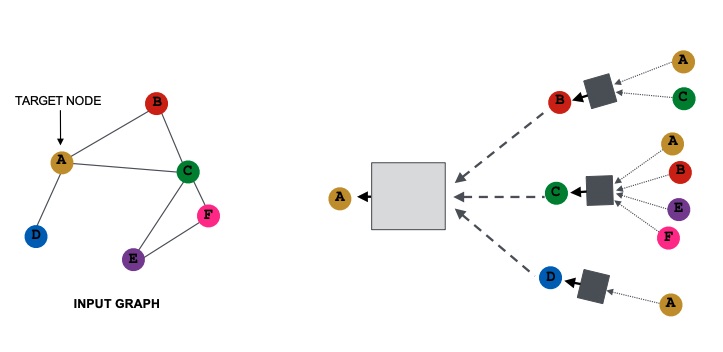
Not all data can be represented using an array. For example the pose of a person is made out of joints and connection, and because of this the most natural way of representing the data is using graphs.
Graph neural networks are the family of networks which data is represented using graph. This includes problems on social networks graphs, or about pose forecasting, 3D objects, protein folding and much more.
Nodes in a graph have no ordering, but they can have some attributes, such as the coordinates in the space (if they represent some kind of structure, like a body), or the content which they refer to (in the case of social networks), and other kind of features.
We want to encode a graph in order to take a decision of some sort. To encode a graph, we need to encode both the node with its attributes, and their connectivities.

This is the GCN Encoder, which should yield a representation of all the input nodes, in such a way that we can use it to make some prediction. As decoder, we can use whatever fits best, for example a Temporal Convolutional Network if we want to do something like forecast human motion.
Note
A graph is defined as following:
- A vertex set
- An adjacency matrix
- A matrix of node features
- Given , we call the set of neighbours of .
Graph Convolutional Networks
In a CNN, each node is arranged on a rigid grid, and when we’re computing a convolution we are just sliding a kernel over the image and computing a element-wise multiplication (the transformation) and summing them up (the aggregation). This produces a representation via an aggregation of local information.
This is exactly what we want to model with a graph, meaning I want to create a representation that is the result of a certain transformation and aggregation of nodes, which depend on the local neighbourhood.
The main difference between image and graph convolution is that a graph doesn’t have an orientation, meaning that the convolutional kernels in an image have specific coefficients for specific pixels (on the right, on the top etc.), while in a graph this doesn’t make sense, and so we need a kernel that works for all the orientations.
As said before, in order to generate the node embedding for each node, we need a transformation of the local information and an aggregation. The transformation is the multiplication with a learned matrix , while the aggregation is the sum. In particular we:
- Take the embeddings of the neighbours nodes
- Compute the average embedding
- Pass the embedding into a fully connected neural network
- This will be the new embedding for the target node.
We do that for each single layer. If we have a multiple layer architecture, we nest the procedure, meaning the output embedding at layer 1 will be the input embedding at layer 2.
We can express this procedure with a formula:
Where:
- : the initial -th layer embeddings are equal to the node features;
- is the average of the neighbour’s embeddings at the previous layer;
- is the activation function;
- is the weights matrix of the FCN, is the matrix that transforms the embedding; These are the only two learnable parameters inside the equation.
- is the total number of layers;
- is the embedding of at layer .
We can write that formula using matrix notation, let’s first define some other notation:
- Let
- Then where A is the adjacency matrix.
- Let be the diagonal matrix where , then we know that also the inverse is diagonal.
- Therefore we can express as
- Let also
With all that notation, we can re-write the update function in matrix form:
Since is sparse, efficient sparse matrix multiplication can be used.
Note
Not all GNNs can be expressed in this matrix form, i.e. when the aggregation function is too complex.
How to train a GNN
In order to train a GNN you have to minimize a loss whee are the node labels and can be a loss if is a real number or cross entropy if it is categorical. are the node embeddings.
In case there are no node label avaliable, we are in the unsupervised setting, and we can use the graph structure as the supervision.
Graph Attention Networks
Since now we’ve seen that embeddings are produced by aggregating neighbourhood information, but we can do better by assigning an arbitrary importance to different neighbours of each node in the graph by learning attention weights across pair of nodes .
In particular, let be the function that computes the attention coefficient based on their messages:
will indicate the importance of ’s message to the node .
We then normalize by passing them trough a softmax function in order to obtain attention weights .
We compute the new node embeddings by performing a sum between the neighbour embeddings weighted by the respective attention weight.
The approach is agnostic to the implementation of , meaning we can use a simple single-layer neural network or something more complex.
A suggestion for a starting point for a GNN layer in practise is the following:
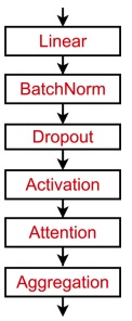
The weights of are trained in conjunction with the parameters of the neural net .
We can also use a multi-head attention, meaning we generate multiple attention scores and then we aggregate them by concatenation, average or summation.
Note
The main benefit of the attention mechanism is the fact that it allows to give different importance values to different neighbours. The approach is also efficient since the computation of attention coefficient can be parallelized across all edges of the graph, and is storage efficient because of the sparse matrix operations.
The over-smoothing problem
The GNNs are stacked in order to be connected. We can also add some skip connections.
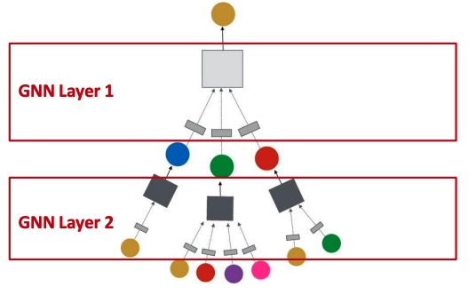
The over-smoothing problem happens when stacking GNN layers like that, since for too many layers the receptive field of each node becomes the whole graph, which means that each node is influenced by all the other nodes and so they all converge to the same value.
In particular, in a -layer GNN, each node has a receptive field of -hop neighbourhood.

We can solve this problem in different ways:
-
Use less but more expressive GNN layers, meaning each transformation and aggregation network can be a deep MLP.
-
Add layers that do not pass messages, such as an MLP before and after the GNN layers which will act as pre and post processing layers.
-
Use skip connections between GNN layers in order to increase the impact of the earlier layers on the final node embeddings.
The intuition behind the latter solution is the fact that skip connection create a mixture of models: with skip connections we have possible paths, since each time the signal can or cannot go trough the skip connection. By doing this, we are creating a mixture of shallow and deep GNNs.
-
Another solution is to insert skip connection between GNN layers, and also from the input to the output.