Logistic Regression

We can define the new loss as:

$${\ell }_{\Theta }(\{x_i,y_i\})=\sum _{i=1}^n(y_i-\sigma (a{x}_i+b){)}^2$$

where the nonlinear $\sigma$ function is called logistic sigmoid

$$\sigma (x)=\frac{1}{1+e^{-x}}$$

The sigmoid function is used to squash the output of $f$ into a value between $(0,1)$. This means that the function has a saturation effect as it maps $\mathbb{R}\to (0,1)$.

Note that this new loss is non-linear with respect to the parameters, since they appear in the non-linear sigmoid function, and it’s also non-convex.

We want the loss to be convex, so we can write a new loss function with this property that will output an high value if the output label is wrong, and a low value if it’s true.

$$c(x_i,y_i)=\{\begin{array}{ll}-\ln (\sigma (a{x}_i+b))& y_i=1\\ -\ln (1-\sigma (a{x}_i+b))& y_i=0\end{array}$$

This works well because if the prediction $\sigma (a{x}_i+b)$ is near the $0$, and the true label is $1$, then $-\ln (\sigma (a{x}_i+b))\to \infty$. On the other hand, if the true label is $0$, then $-\ln (1-\sigma (a{x}_i+b))\to 0$.

We can rewrite the function on a single line:

$$c(x_i,y_i)=-y_i\ln (\sigma (a{x}_i+b))-(1-y_i)\ln (1-\sigma (a{x}_i+b))$$

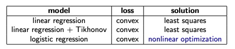
The function is still non-linear with respect to the parameter, but is convex.

The loss for the entire dataset will be:

$${\ell }_{\Theta }(\{x_i,y_i\})=\sum _{i=1}^{n}c(x_i,y_i)$$

Closed form solution for Logistic Regression

As we did for the Linear Regression case, we want to find a closed form solution by putting the gradient of the loss equal to zero. Since the loss is convex, we will find the global minimum.

Show how to find the right theta

Finding theta such as $\nabla_\Theta\ell_\Theta = 0$

We set the gradient to zero and we want to solve it for $\Theta$.

$$
\begin{align}
\nabla_{\Theta} \sum_{i=1}^n y_i \ln \left(\sigma\left(a x_i+b\right)\right)+\left(1-y_i\right) \ln \left(1-\sigma\left(a x_i+b\right)\right)=0 \\

\end{align}
$$

Since the gradient operation is linear, the gradient of the summation is just the sum of the gradient of each term, so we can consider just the gradient of a single term.

$$
\begin{align}
\nabla_{\Theta}  y_i \ln \left(\sigma\left(a x_i+b\right)\right)+ \left(1-y_i\right) \ln \left(1-\sigma\left(a x_i+b\right)\right)
\\
\nabla_{\Theta}  y_i \ln \left(\sigma\left(a x_i+b\right)\right)+\nabla_{\Theta} \left(1-y_i\right) \ln \left(1-\sigma\left(a x_i+b\right)\right)
\\
y_i\nabla_{\Theta}   \ln \left(\sigma\left(a x_i+b\right)\right)+\left(1-y_i\right)\nabla_{\Theta}  \ln \left(1-\sigma\left(a x_i+b\right)\right)
\\
y_i\nabla_{\Theta} \underbrace{\ln \left(\sigma\left(a x_i+b\right)\right)}_{f(g(h(\Theta)))}+\left(1-y_i\right)\nabla_{\Theta}  \ln \left(1-\sigma\left(a x_i+b\right)\right)
\end{align}
$$

We can apply the chain rule in order to take the derivative of the composition of three function.

$$
\begin{align}
\frac{\partial}{\partial a}f(g(h(a,b))) = \frac{\partial f}{\partial g} \cdot \frac{\partial g}{\partial h} \cdot \frac{\partial h}{\partial a}
\end{align}
$$

We solve the first partial derivative:

$$
\begin{align}
\frac{\partial h}{\partial a} =\frac{\partial}{\partial a} ax_i+b = x_i 
\end{align}
$$

We solve the second partial derivative:

$$
\begin{align}
\frac{\partial g}{\partial h} =\frac{\partial \sigma(ax_i+b)}{\partial (ax_i+b)} = \frac{\partial}{\partial\left(a x_i+b\right)} \frac{1}{1+e^{-\left(a x_i+b\right)}} = \frac{e^{-\left(a x_i+b\right)}}{\left(1+e^{-\left(a x_i+b\right)}\right)^2} \\
=
\frac{1}{1+e^{-\left(a x_i+b\right)}} \frac{e^{-\left(a x_i+b\right)}}{1+e^{-\left(a x_i+b\right)}} \\
= \frac{1}{1+e^{-\left(a x_i+b\right)}} \frac{\left(1+e^{-\left(a x_i+b\right)}\right)-1}{1+e^{-\left(a x_i+b\right)}} \\
= \frac{1}{1+e^{-\left(a x_i+b\right)}}\left(1-\frac{1}{1+e^{-\left(a x_i+b\right)}}\right) \\
=
\text { - } \sigma\left(a x_i+b\right)\left(1-\sigma\left(a x_i+b\right)\right)
\end{align}
$$

Finally we solve the third partial derivative:

$$
\begin{align}
\frac{\partial f}{\partial g} =
\frac{\partial \ln \left(\sigma\left(a x_i+b\right)\right)}{\partial \sigma\left(a x_i+b\right)} =\frac{1}{\sigma\left(a x_i+b\right)}
\end{align}
$$

Plugging everything in the equation at $(6)$:

$$
\begin{align}
\frac{\partial}{\partial a} f(g(h(a, b)))=\frac{1}{\sigma\left(a x_i+b\right)} \cdot \sigma\left(a x_i+b\right)\left(1-\sigma\left(a x_i+b\right)\right) \cdot x_i \\
= \left(1-\sigma\left(a x_i+b\right)\right) \cdot x_i
\end{align}
$$

And so:

$$
\frac{\partial}{\partial a} \ln \left(\sigma\left(a x_i+b\right)\right)=\left(1-\sigma\left(a x_i+b\right)\right) x_i
$$

Now this should be done also for the left ther of $(5)$, and everything should be repeated w.r.t. $b$ in order to compute the full gradient.

We can see from a part of the partial derivative which consistutes the gradient:

$$\frac{\partial }{\partial a}\ln \left(\sigma \left(a{x}_i+b\right)\right)=\left(1-\sigma \left(a{x}_i+b\right)\right)x_i$$

that the system of equations that we have when we set the gradient to $0$ wouldn’t be a linear system, since both $a$ and $b$ are involved in a non-linear function and so it cannot be easily solved.

Furthermore, the system is a transcendental equation, because it involves the exponential function inside the sigmoid function, which definition is the sum of an infinite series. Because of that, an analytical solution, and so a closed form solution, doesn’t exist.

In order to find the parameters that minimize the loss, we need to use an iterative method like stochastic gradient descent.