Recurrent Neural Networks (RNN)

RNN is an architecture based on an internal state, which gets updated as the sequence is processed.

The output $y$ is a function of not only the input $x$ but also of the recurrent module.

We can express the general formula for the RNN as:

$$\underset{\text{new state}}{\underbrace{h_t}}=\underset{\text{function with parameters }W}{\underbrace{f_W}}(\underset{\text{previous state}}{\underbrace{h_{t-1}}},\underset{\text{input vector}}{\underbrace{x_t}})$$

In a more specific way:

$$h_t=\tanh (W_{hh}{h}_{t-1}+W_{xh}{x}_t)=\tanh \left(W\left[\begin{array}{c}{h}_{t-1}\\ x_t\end{array}\right]\right)$$

And then we compute the output as:

$$y_t=W_{hy}{h}_t$$

Computational graphs

In the Vanilla RNN, the hidden state $h$ consists of a single vector.

Note that there is always just a single set of parameters $W$ for the entire sequence processing.

We can use RNNs for all the types of sequence problems we’ve seen so far.

Many to Many

In the many-to-many case, at each step an output is produced and the loss is updated.

Many to One

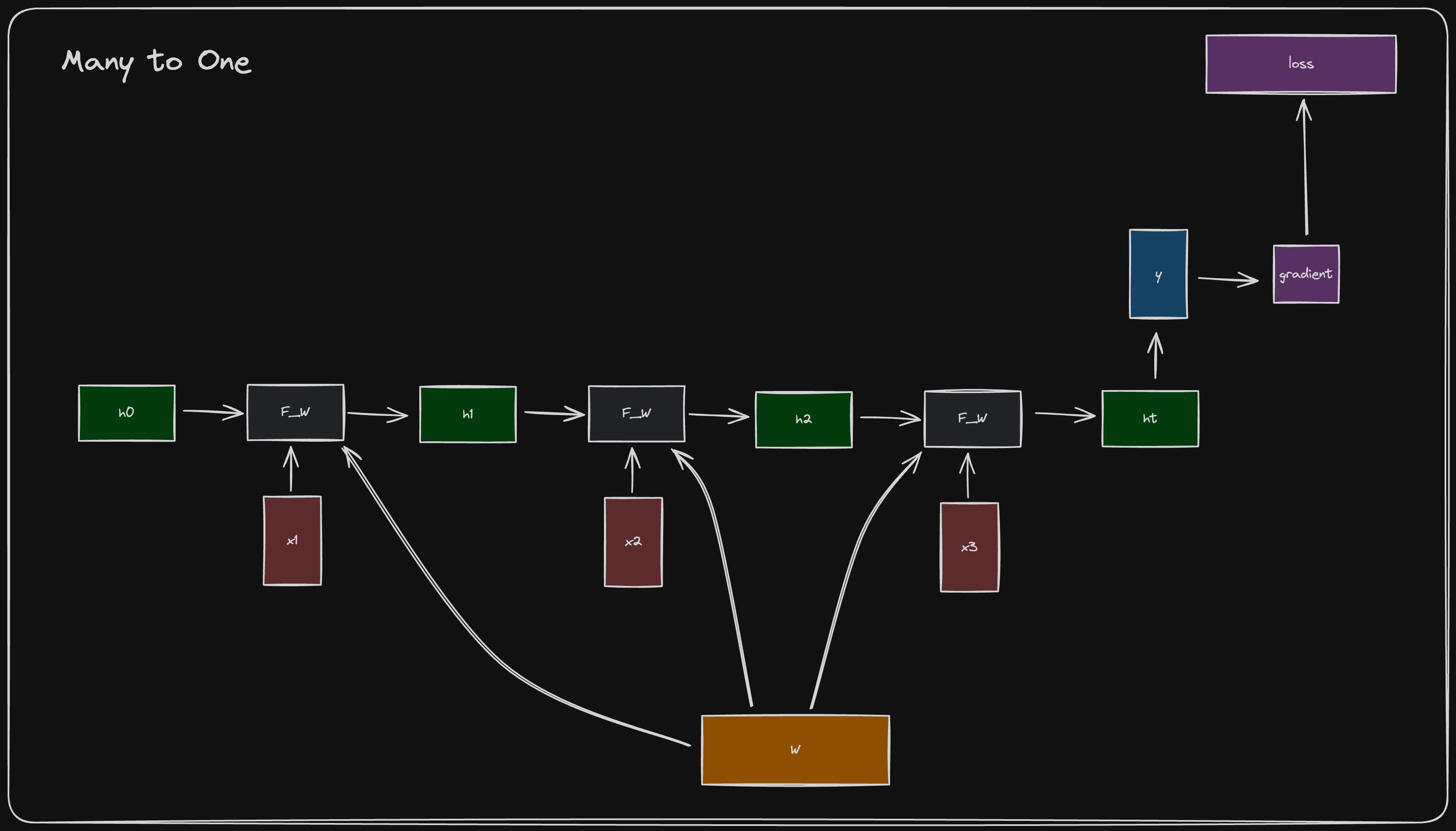
In the many-to-one case, just a single output is produced, and a single loss is computed at the end.

One to Many

In the one-to-many case, we just have a single input $x$. The problem is that we have to insert an input for all the other steps. Here we have two solutions:

• Just put a $0$. This is not the best solution since we are putting some data that we invented.
• Put $y_{t-1}$. This is a more reasonable solution and makes the RNN autoregressive, meaning the output at time step $t$ is given as input for the time step $t+1$.

Many to One + One to Many

If we want to do a Many to Many, we can also first encode the input sequence in a single vector with a many-to-one RNN, then we take the single vector and produce a sequence as the output with a one-to-many RNN.

Example: Character-level Language Model Sampling

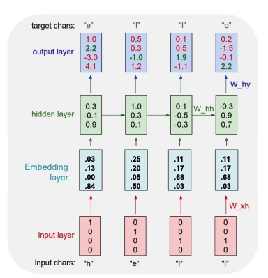
Most of the times the input goes first into an embedding layer, which produces an embedding, which then is passed to the hidden layer to produce an output. This is an autoregressive modelling, since each time we predict a new character from the current character and the current hidden state, and then feed the produces character to the next input.

Similarly for image, they can be embedded with the use of a CNN, which will produce a logits vector. We can then apply the RNN on the logits and perform our task (such as image captioning).

Note

Since the model tries to not be wrong, regarding image captioning it may produce some oversimplified captions such as “a picture of a cat”.

The past context is summarized inside of the hidden unit. If the context (past) is too long, the hidden state will begin to forget it, because it’s not as powerful. Transformers will be able mitigate this problem.

Ground Truth Forcing

Also known as “teacher forcing”, ground truth forcing consists in inputting computing the loss between the predicted token and the ground truth, and input the ground truth (instead of the model’s own prediction) in the next prediction step.

The main advantage of ground truth forcing is to make the learning process more stable, since if the model is trained with its own prediction, if a prediction at step $t$ is very wrong, the ones at step $t^{\prime }>t$ will be negatively affected. This doesn’t happen if we input the ground truth token.

This of course can be done only at train time, and at inference time the model predictions are given in input to the next steps.

Truncated backpropagation

We’ve seen how in a Vanilla many-to-many RNN each output contributes to the same loss, which becomes expensive fore long sequences, because of the many steps of chain rule that we have to apply.

A solution to this problem is truncated backpropagation, where the forward pass is done as usual, but the backpropagation is done only for a smaller number of steps in the past. This operation will produce a gradient for each segment. Note that the gradient refers to the same $W$.

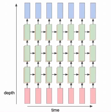
Multilayer RNNs

It’s possible to have multiple layers of a RNN

RNN Gradient Flow and long-term dependencies

Learning long-term dependencies with gradient gradient descent is difficult, because the gradient tends to vanish for long sequences. RNNs suffer from this phenomenon, let’s see why does this happen in detail.

In particular, we can see that the hidden $h_t$ at time $t$ is the result of:

$$h_t=\tanh \left(W_{hh}{h}_{t-1}+W_{xh}{x}_t\right)=\tanh \left(W\left(\begin{array}{c}{h}_{t-1}\\ x_t\end{array}\right)\right)$$

This means that the backpropagation form $h_t$ to $h_{t-1}$ multiplies by $W$.

The derivative is:

$$\frac{\partial h_t}{\partial h_{t-1}}={\tanh }^{\prime }\left(W_{hh}{h}_{t-1}+W_{xh}{x}_t\right)W_{hh}$$

We also know that the derivative of the loss w.r.t. $W$ is the summation of the derivative of the loss at time $t$ wrt to $W$:

$$\frac{\partial L}{\partial W}=\sum _{t=1}^T\frac{\partial L_t}{\partial W}$$

If we’re considering the last of the losses ($L_T$) and the first $W$, we can obtain the formula with the chain rule:

$$\frac{\partial L_T}{\partial W}=\frac{\partial L_T}{\partial h_T}\frac{\partial h_t}{\partial h_{t-1}}\dots \frac{\partial h_1}{\partial W}$$

Note that

$${\tanh }^{\prime }(x)=1-{\tanh }^2(x)$$

and sine $\tanh (x)\in [-1,1]$, ${\tanh }^{\prime }(x)$ will be in the range $[0,1]$, and so ${\tanh }^{\prime }$ is always $<1$.

Because of this, if we have an higher $T$, then $\frac{\partial L_T}{\partial W}$ will be closer and closer to $0$, since we are multiplying by numerous factors in $[0,1)$. This is the vanishing gradients problems, which causes the network to stop learning.

If we don’t use the $\tanh$, we will have a $W_{hh}^{T-1}$ (where $T^{-1}$ is the exponent of which we raise $W$). Here, if the largest singular value of the matrix $W$ is greater then $1$, we get exploding gradients, otherwise we get vanishing gradients again, because of the matrix exponentiation.

We can clip the gradients (scale the gradient if its norm it’s bigger than a decided threshold) in order to avoid exploding gradients, but we need to modify the architecture in order to solve the vanishing gradient problem.

The most basing way of solving this is by using skip connections, in order for the network to not always backpropagate through $W$.

💡 In conclusion, RNNs are good since they can:

• Process any input length
• Maintain an internal state
• Model size doesn’t increase for longer input
• Same weights applied at each timestep, meaning there is a symmetry in how the inputs are processed.

RNN do have some limitations:

• Recurrent computation is slow
• Difficulty in training for long sequences