Transformers

Useful Resources

• Attention Is All You Need - Paper Explained
• The Illustrated Transformer – Jay Alammar – Visualizing machine learning one concept at a time.
• Attention Is All You Need - Arxiv.org

Transformers are the current best sequence model for a variety of tasks, and they outperform LSTMs on pretty much everything, but their architecture is very complex and the training demands a lot of data.

Attention Mechanism

To better understand the problem with RNNs and LSTMs, let’s consider the example of language translation. With RNNs, the hidden state represents a compressed state of what the machine thinks the meaning of the sentence is. Each time we produce a word in the target language, the internal state length is always the same. So since we don’t know what the size of the output sentence be a priori (sampled until the EOS token is sampled), with long output sentences the model will forget the dependencies.

Note

This problems also occurs with image captioning via a CNN + RNN, when we extract the features from an image and then we feed the logits to the RNN, the output sequence length is unknown and we have the same problem.

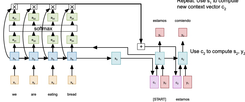
Attention-based mechanism compute the vector each time they need to sample a new word, which will be different according to what the word may depend on.

Attention allows to compute a score vector that tells how much the past decoder state relates to the current decoder state. From this score vector it’s possible to compute some attention weights, which gives to each token a weight. We then softmax those tokens and element-wise multiply them with the current hidden states, in order to have an hidden state that is scaled based on the attention weights relative to the current word. In this way, the context should encode which part of the input sentence is more relevant to sample the next word. We do that each time we need to sample a word.

All those operations are fully differentiable, and so we can run backpropagation through them, which allows the model to learn the attention weights. The attention is in fact just a MLP which is trained in an unsupervised manner (otherwise it would be required to have labels for the attention for each sentence).

Different types of Attention

Attention mechanisms have been studied a lot during the years, and there a lot of variations to it. The variations are in the way the attention weights are computed.

Let $x$ be the input sequence. In the typical attention layer, there are three actors:

• Query $q$: the vector that produces the attentions scored when multiplied with the key vector $k$. In the general attention mechanism, $q$ is an external vector that has to be given to the layer. This step is also called alignment.

• Key $k$: it’s computed from the input vector $x$ by a multiplication with a learnable matrix $W_k$.

  $$k=x{W}_k$$

• Value $v$: it’s computed from the input vector $x$ by a multiplication with a learnable matrix $W_v$.

  $$v=x{W}_v$$

The two most famous attention mechanism (before the scaled dot-product attention) are:

• Dot-Product Attention:

  $$\text{Attention}(Q,K,V)=\text{softmax}\left(Q{K}^T\right)V$$

• Additive Attention (aka ****Bahdanau Attention): It uses a feed-forward network with a single hidden layer in order to compute the compatibility function.

  $$\text{Attention}(Q,K,V)=\text{softmax}(e)V$$

  where $e=\tanh (W_{Q}Q+W_{K}K)$ with $W_Q$ and $W_K$ being learnable weight matrices.

Scaled Dot-Product Attention

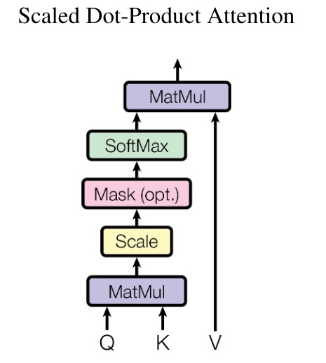
The attention mechanism proposed in the Attention is All You Need paper, that is the one used in the Transformer architecture, is the Scaled Dot-Product Attention, defined as following:

$$\text{Attention}(Q,K,V)=\text{softmax}\left(\frac{Q{K}^T}{\sqrt{d_k}}\right)V$$

This mechanism is the same as the Dot-product attention, but with the addition of the scaling factor $\frac{1}{\sqrt{d_k}}$, since the standard Dot-product attention performs worse when $d_k$ increases, probably because the dot products grows large in magnitude, pushing the softmax function into regions where it has very small gradients.

Multi-head attention

Instead of performing a single attention function with $d$-dimensional keys, values and queries, they found to be more beneficial perform $h$ attention functions with $h$ different learned matrices. The final result will produce $h$ attention scores, which will then be concatenated and projected into a $d$ dimensional vector with the use of a learned matrix $W^O$.

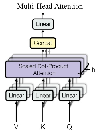
Multi-head attention allows the model to jointly attend to information from different representation subspaces at different positions.

In the example of Natural Language Processing, this means that one head may be focusing on “who did the action”, while another head on “what action was done”

The formula for the multi head attention is the following

$$\begin{array}{rl}\mathrm{MultiHead}(Q,K,V)& =\text{Concat}\left({\text{head}}_1,\dots ,{\text{head}}_{\mathrm{h}}\right)W^O\\ \text{ where }{\text{head}}_i& =\text{Attention}\left(Q{W}_i^Q,K{W}_i^K,V{W}_i^V\right)\end{array}$$

Where:

• $W_i^Q\in {\mathbb{R}}^{d\times d_k}$
• $W_i^K\in {\mathbb{R}}^{d\times d_k}$
• $W_i^V\in {\mathbb{R}}^{d\times d_v}$
• $W_i^O\in {\mathbb{R}}^{h{d}_v\times d}$

Self Attention

Self attention differs from in the fact that queries are not given, but are computed from the input vectors $x$ with a multiplication for a learnable matrix $W_q$.

$$q=x{W}_q$$

It’s called self-attention because the input $x$ is the only input needed to generate the queries, keys and values.

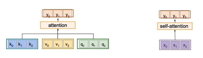
General attention vs self-attention

Positional Encoding

The limitation with the current approach is the that the decoder doesn’t treat the hidden states $h_i$ as ordered sequences, which in sequential modelling plays an essential role.

In order to solve this, we can use positional encodings.

The idea behind positional encoding is to define a function $pos(t)$ that takes in input the time-step $t$ and outputs an unique encoding for each time-step, which encodes the position in of the token in the sentence. It should generalize to longer sentences and should be deterministic.

We also want $pos(t)$ to have a consistent distance between any two time steps, and it should be deterministic.

We have two main options:

• Learn the parameters to use for $pos(t)$ for each $t\in [0,T)$, and insert each possible value in a lookup table with $T\times d$ parameters.
• Design a fixed function for $pos(t)$.

The first one works well, but the second one is desired, since we don’t have to learn anything.

In particular, the second option is the most used, with $pos(t)$ defined as following:

$$pos(t)={\left[\begin{array}{c}\sin \left({\omega }_1\cdot t\right)\\ \cos \left({\omega }_1\cdot t\right)\\ \sin \left({\omega }_2\cdot t\right)\\ \cos \left({\omega }_2\cdot t\right)\\ ⋮\\ \sin \left({\omega }_{d/2}\cdot t\right)\\ \cos \left({\omega }_{d/2}\cdot t\right)\end{array}\right]}_d\in {\mathbb{R}}^d$$

Where ${\omega }_k=\frac{1}{10.000^{2k/d}}$.

Since sine and cosine are periodic functions, we can alternate between sine and cosine and each time give a period that is in function of $k$.

The maximum count that I can have is $\frac{10.000}{2\pi }\approx 1.600$, and then the counting restarts. The $10.000$ is chosen because the $1.600$ is assumed to be a good compromise.

If the $t$ is small (which happens in the last positions of the vector) the $pos$ function fluctuates very fast, for an higher $t$ (which is the case for the first positions of the vector), it fluctuates slowly. This allows us to encode the position of the token in the sentence, since all the $pos$ with different $t$ are different.

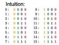
The intuition is that this will behave similarly to binary counting, meaning functions with a smaller period (the last positions in the vectors) will oscillate more frequently, while the ones with an higher period will oscillate rarely.

Once we have the encoding for each token in the sentence, we just add it to the token embedding. This will allow the model to distinguish two equal tokens in different position.

Masked Self-Attention

During the output generation, because the task is autoregressive, we need to make sure that the self attention mechanism cannot put any attention on the future tokens. We can do that by masking the attention scores in the alignment phase, setting the left part of the diagonal to $-\infty$, in order for it to be $0$ once the softmax operation is performed.

This is done only in the decoder, which is the block that is responsible for the output generation. In the encoder this isn’t necessary since it takes in input the entire sentence at once, and there is no autoregression.

Transformer Network

Now that we have the concept of Attention and Self-Attention, we can define what a transformer network is.

Introduced in the paper “Attention is all you need” by Vaswani et al. in 2018, a transformer is an architecture that only uses self-attention blocks in order to perform the task. This is a historical step in the field of computer science, since transformers are capable of working with much longer sentences and with much bigger contexts, which was a the downside of RNNs and LSTMs.

Architecture Details

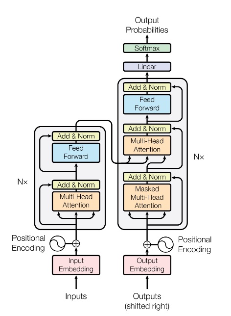
The encoder is composed of a stack of $N=6$ identical layers. Each layer has two sub-layers. The first is a multi-head self-attention mechanism, and the second is a simple, position- fully connected feed-forward network. There is a residual connection around each of the two sub-layers, followed by layer normalization. That is, the output of each sub-layer is $\text{LayerNorm}(x+\text{Sublayer}(x))$, where $\text{Sublayer}(x)$ is the function implemented by the sub-layer itself.

The decoder is also composed of a stack of $N=6$ identical layers. In addition to the two sub-layers in each encoder layer, the decoder inserts a third sub-layer, which performs multi-head attention over the output of the encoder stack (in an autoregressive manner).

Similar to the encoder, we employ residual connections around each of the sub-layers, followed by layer normalization. We also modify the self-attention sub-layer in the decoder stack to prevent positions from attending to subsequent positions. This masking, combined with fact that the output embeddings are offset by one position, ensures that the predictions for position i can depend only on the known outputs at positions less than $i$.

It’s important to know that only the final encoder output goes into each decoder multi head attention layer.

---

Transformers are a very capable type of models which can be pre-trained on a huge corpus of text, and then can be fine-tuned on a smaller dataset in order to perform well on a particular domain.

Differently from LSTMs, in the transformer architecture we can better see the separation of concerns in learning. For example, in the context of language translation, the encoder will learn “what is the origin language, and what is context”, while the decoder will learn “how to map the origin language words into the target language words”.

Vision Transformers

Vision transformers are transformers networks that are used on images. Before those, transformers could work on images by taking in input the logits obtained with CNNs.

We can divide images into patches of equal size and input those patches to the transformer encoder, and those will be treated as sequences. It has been shown that ViT have better performances than ResNets.

Relative Self Attention

In music you need to encode a lot of information for each node, such as the type of node, its velocity, then it’s pressed and when it’s released. A way of doing this is to use MIDI representation.

Let’s say that we want to build a model that, given an initial model, returns a set of nodes that continue that motif. To do that we need to maintain a long term relationship, since notes in the future depends on the initial notes, in order to not lose the general motif.

First of all, speaking of attention in music has a lot of sense, since rhythms in music are very self-similar. Because of that, looking at the right set of notes in the past allows you to generate a good sounding future set of notes.

Models like Performance RNNs and LSTMs tend to forget the initial motif after some time, since they struggle to encode long term dependencies. Same thing happens with a transformer with simple self-attention.

Note

Still today, encoding long-term dependencies is still challenging and a very active research topic.

In order to solve this problem, we need relative self-attention, which is another way of encoding the positions of the points in the sentence, generally more performant than positional encoding. (Remember that the Transformer, without positional encoding, it’s completely invariant to the sentence ordering).

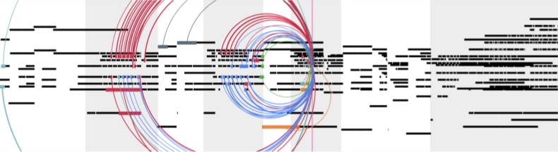
In this figure, the arcs represent what past notes the model looks in order to generate a new note. We can see that it makes sense, since it’s currently predicting a chorus, and to do that it’s looking at notes in the previous two choruses.

If we look at plain attention, that’s just a weighted average, weighted by the attention weights. Convolution behave in a similar manner: the kernel parameters are the weights for the weighted average.

Convolutions and attentions, in particular multi-head attention, can be brought together.

The model should be able to learn the offset between the current note and the note to put attention on.

In particular, the self attention is computed (for each head $h$ omitted for clarity) as:

$$Z=\text{Softmax}\left(\frac{Q{K}^T}{\sqrt{D}}\right)V$$

which is timestamped by a positional encoding.

On the other hand, the relative self-attention is computed as:

$$Z=\text{Softmax}\left(\frac{Q{K}^T+Qf(E_{rel})}{\sqrt{D}}\right)V$$

Where $Qf(E_{rel})$ is a shift that is function of the query matrix $Q$ and a function $f$ that depends on the learned relative position embedding $E_{rel}$.

Relative Self-Attention and Graphs

Todo

Still work in progress