FDS - Concepts for the Final quiz

Concepts for the Final quiz

Basic graphics and CV

• Kernel convolution

  Kernel convolution denotes an operations that is done over an image using a small matrix called kernel (or filter).

  Formally, let $I$ be the image of shape $m\times n$ and let $g$ be the kernel of size $k\times l$, then the pixels of the final image $f$ are defined as:

  $f[m,n]=I\otimes g={\sum }_{k,l}I[m-k,n-l]g[k,l]$.

  We can also apply $I[m+k,n+l]$ with the mirrored kernel.

• Separability principle

  The separability principle tells us that if a filter is separable it means that it can be written as the product of two or more lower dimension filters.

  For example a 2D filter can be expressed as two 1D filter. The image is first convolved on all of the row and then on all of the columns.

  The convolution of two 1D filter is more efficient than a single convolution with a 2D filter.

  Generally a filter is separable if its equation, which depends on $x$ and $y$, it’s factorizable in two equation that depend one on $x$ and one on $y$.

• Average filters

  Some of the average filters are:

  • Box filter: is a type of average filter that replace each pixel with the average of its neighbors, giving all of them the same weight.
  • Gaussian filter: it’s similar to the box filter, but gives the nearest neighbors more weight, this results in a blurred image with more details. The weight can be controlled by the $\sigma$ value. When the $\sigma$ is larger, the kernel gets larger and the image is smoother, and vice versa otherwise.

• Sharpening

  Sharpening it’s a type of filter that enhances the changes in the color intensity of the image, resulting into a more detailed picture.

  It’s possible to sharpen an image by doubling all the pixels and then subtracting the blurred image.

• Gaussian pyramid

  A gaussian pyramid is a type of multi-scale image representation in which each image in the upper part of the pyramid is obtaied by smoothing the previous image with the Gaussian filter before scaling it down.

  Smoothing the image before the downscale is essential in order to mantain as much information as possible. Subsampling without smoothing could also lead to aliasing.

  During this procedure the average of pixels is preserved, but the higher frequencies are lost.

  Multi-scale image representation is useful because the same image can enhance different information ad different scales.

• Edge detection

  Edge detection is a convolutional operation that allows to generate an image that enhances the edge zones in a certain direction.

  We can see how edge detection works by considering the horizontal edge of a single line in the image. If we take the derivate of the curve that describes that line, the derivative curve will have a peak where the edge is located.

  We can implement the first derivative as a convolution with the 1D kernel $[-1,1]\text{ or }[-1,0,1]$.

  In order to remove some noise it’s better to first smooth the image with a gaussian filter. To associate the two operations (since the derivative is a associative operation), it’s possible to convolve the image with the derivative of the gaussian in order to obtain the edge in a more efficient way. These type of kernels are called Sobel kernels ($G_x$ and $G_y$).

  Images are in 2D, so in order to perform edge detection we have to compute the derivative for each line in each direction. In this case the kernel for the $x$ direction $D_x$ and the kernel for the $y$ direction $D_y$ are fined as following (different from sobel kernels):

  $$\begin{gathered} D_x=\frac{1}{3}\left[\begin{array}{ccccc}-1& & 0& & 1\\ -1& & 0& & 1\\ -1& & 0& & 1\end{array}\right], \\ {D}_y=\frac{1}{3}\left[\begin{array}{ccccc}-1& & -1& & -1\\ 0& & 0& & 0\\ 1& & 1& & 1\end{array}\right] \end{gathered}$$

  It’s also possible to perform edge detection by computing the second derivative of each line of the image, since an edge would be modeled by a zero crossing of the curve. This is useful since it better marks the intensity of the pixels around the image. The kernel in this case is $[1,-2,1]$.

• Canny edge detector

  Canny edge detector is an edge detector operator that proceeds in the following way:

  1. Smooth the image with a gaussian filter
  2. Find the intensity gradient of the image by convolve it with a Sobel kernel to enhance the edges in both directions;
  3. Apply non-maximum suppression in order to thinnen the edges of the image.
  4. Apply thresholding in order to remove some edges that may be caused by noise.
  5. Track the missing edges by using hysteresis.

• Laplacian pyramid

  The laplacian pyramid is a multi-scale image representation in which each image $L_i=G_i-\text{expand}(G_{i+1})$. The pyramid is represented by the series of images $L_1,L_2,\dots ,L_n$.

  The $L_i$ difference is approximately equivalent to the convolution between the image and laplacian of the Gaussian kernel.

  The laplacian operator is defined as ${\nabla }^{2}f=\frac{{\partial }^{2}f}{\partial x^2}+\frac{{\partial }^{2}f}{\partial y^2}$ , and the kernel convolution operation between the image and the gaussian kernel is defined as ${\nabla }^2(G\otimes f)={\nabla }^{2}G\otimes f$.

• Color histograms and their comparison

  It’s possible to compare images by extracting a certain histogram,f or example the colo histogram, that is the luminance histogram (describes the distribution of pixel intensity) applied to all three channels, and then compute the distance between those histograms.

  If the color in in RGB, we can build the 3D joint color histogram with a cube of shape $(l,l,l)$ where $l$ is the width of the image, and where at the $(r,g,b)$ coordinate there is the number of pixels with that combination of values.

  There are many distance techniques that can be used, here the most common (note that the histogram has to be normalized first):

  • Intersection: defined as $\bigcap (Q,V)={\sum }_{i}min(q_i,v_i)\in [0,1]$, it measures the common part of both histograms.
  • Euclidean distance: defined as $d(Q,V)={\sum }_i(q_i-v_i{)}^2\in [0,\infty ]$, focuses more on the difference between the distance, but is not very discriminant since all cells are weighted equally.
  • Chi-square: defined as ${\chi }^2(Q,V)={\sum }_i\infty (q_i-v_i{)}^2{q}_i+v_i\in [0,\infty ]$, similar to the euclidean distance but the different cells are weighted differently. Two image with the same colors are more similar.

• Nearest-Neighbour strategy

  Is a simple algorithm to get the list of most similar images from a certain query image.

  It works by building a set of histograms for each known object (gallery), build the histogram for the test image and then order the histograms in the gallery according to the highest similarity score. The first of this list is accepted as the most similar if the score is above the threshold, otherwise it means that no image is similar enough.

  It’s possible to consider only $k$ of those nearest neighbours. The name of this technique then becomes $k$-nearest neighbours.

ML Methods for prediction

• Linear regression

  It’s used to fit a line which equation allows to predict new values. The basic case is when we have just one feature ($n=1$) with $m$ training examples.

  $x$ is the training example (independent variable) and $y$ is the target variable (dependent variable).

  Both the input $x$ and the output $y$ can be discrete or continuous values.

  The line has equation $h_{\theta }={\theta }_0+{\theta }_{1}x$.

  We can fit the parameters by optimizing the cost function with optimization methods like gradient descent.

  The cost function in this case is the sum of squared errors:

  $J({\theta }_0,{\theta }_1)=\frac{1}{2m}{\sum }_{i=1}^m(h_{\theta }(x^{(i)})-y^{(i)}{)}^2$

• Multivariate linear regression

  It’s the generalized case of linear regression, in case we have more than just one feature, but always one target.

  The line we want to fit now has equation $h_{\theta }={\theta }_0+{\theta }_1{x}_1+{\theta }_2{x}_2+...+{\theta }_n{x}_n={\sum }_{i=0}^n{\theta }_i{x}_i={\theta }^{T}x$.

  In the general case we can express the equation as $h_{\theta }(x)={\theta }^{T}x$ where both $\theta$ and $x$ are vectors.

• Polynomial regression

  It’s used in the same way as linear regression, but when the examples cannot be separated by a line, and a curve is needed.

  We can add non-linear variation of the features, and the equation can be something like this: $h_{\theta }(x)={\theta }_0+{\theta }_{1}x+{\theta }_2{x}^2+{\theta }_3{x}^3$.

• Locally weighted linear regression

  It’s a variation of polynomial regression in order to give more weight to the data points near the one that has to be predicted.

  The weight is computed as following: $w^{(i)}=\exp \left(\frac{-\Vert x^{(i)}-x\Vert }{2{\tau }^2}\right)$.

  Tau ($\tau$) is an hyperparameter and represent the bandwidth, meaning how wide the datapoint set from which to compute the weight has to be.

  The weight is computed ad test time, since $x$ is the equation we want to test. The equation that has to be minimized becomes:

  $$\sum _{i=1}^m{w}^{(i)}(y^{(i)}-{\theta }^T{x}^{(i)}{)}^2$$

Classifiers

• Logistic regression with linear boundaries

  Logistic regression fits a line that best divide the two classes of examples. The basic version is used for binary classification, meaning there could only be two classes.

  The indipendent variable $x$ can be discrete or continuous, the output is a binary (or multinomial) value, so it’s necessarily discrete.

  The equation is the same as the linea regression one, but we apply the sigmoid in order to limit the range of the returned value to $[0,1]$.

  $h_{\theta }(x)=g({\theta }^{T}x)$ where $g(z)=\frac{1}{1+e^{-z}}$.

  We then set a treshold of prediction accordingly.

  In terms of probability, we can also write that $h_{\theta }(x)=P(y=1|x;\theta )$, meaning that the result of the function is the probability that $x$ is in the positive class.

  We can use apply gradient descent to the likelihood or gradient ascent to the log-likelihood to fit the parameters.

  The likelihood in this case is described as: $L(\theta )={\prod }_{i=1}^m{h}_{\theta }(x^{(i)}{)}^{y^{(i)}}(1-h_{\theta }(x^{(i)}){)}^{1-y^{(i)}}$. We can take the log-likelihood from this and its derivative would be: $\frac{\partial }{\partial {\theta }_j}\ell (\theta )={\sum }_{i=1}^m\left(y^{(i)}-h_{\theta }(x^{(i)})\right)x_j^{(i)}$.

• Logistic regression without linear boundaries

  In case we cannot divide the two classes with a line, we can use the same approach seen on polynomial regression in order to fit a curve. The only thing needed is to pass the polynomial regression function to the sigmoid.

• Multinomial logistic regression (Softmax regression)

  Softmax regression it’s used for multinomial classification, meaning if we have more than two classes.

  It uses the softmax function $\sigma (x{)}_i=\frac{e^{x_i}}{{\sum }_{j=1}^K{e}^{x_j}}$ that returns the probability of the sample $x_i$ being in the $i$-th class.

  The function $h_{\theta }(x)=$ $P(Y=K|x;\theta )$ returns the vector of size $n\times m$ where in position $i$ there is the probability that $x$ belongs to the $i$-th class. The vector sums to $1$.

  We can fit the parameters by computing the log-likelihood and then using MLE with methosds like gradient ascent.

• Gaussian Discriminant Analysis

  GDA is a generative learning classifier that is used to perform binary classification. Since it’s generative, it learns $P(x|y)$ instead of learning $P(y|x)$ like discriminative learning models.

  Once we have $P(x|y)$ we can obtain $P(y|x)=\frac{P(x|y)P(y)}{P(x)}$ following Bayes rule.

  With the assumption that $P(x|y)$ is gaussian, the GDA fits two multivariate gaussian, one for each class, and the separation between the two implies a decision boundary similar to the one fitted by logistic regression. The feature vectors $x$ in this case are continuous.

  GDA is parametrized by:

  • ${\mu }_0\in {\mathbb{R}}^n,{\mu }_1\in {\mathbb{R}}^n$, that is the mean relative to each class;
  • $\Sigma \in {\mathbb{R}}^{n\times n}$, that is the covariance matrix of the two classes;
  • $\varphi =P(y=1)$, that is the probability of the true case.

  In generative learning algorithms the joint likelihood is defined as $L(\varphi ,{\mu }_0,{\mu }_1,\Sigma )={\prod }_{i-1}^{n}P(x^{(i)},y^{(i)};\varphi ,{\mu }_0,{\mu }_1,\Sigma )={\prod }_{i-1}^{n}P(x^{(i)}|y^{(i)})P(y^{(i)})$, differently from the one of discriminative learning algorithms ($L(\theta )={\prod }_{i=1}^{n}P(y^{(i)}|x^{(i)};\theta )$)

  The mean and covariance are estimated using the maximum likelihood estimate (by differentiating the log-likelihood and putting the derivative equals to zero, since we are sure that the equation is differentiable, not like other methods).

  To predict a value, we can get the ${\mathrm{argmax}}_{y}P(y|x)={\mathrm{argmax}}_y\frac{P(x|y)P(y)}{P(x)}$ that’s equals to getting ${\mathrm{argmax}}_{y}P(x|y)P(y)$ since the denominator is a constant and can be deleted for computational advantages.

  GDA is much more efficient since it doesn’t have to optimize a cost function, but it performs well only if the data is gaussian.

  If we don’t want a linear classifier, we can use QDA, that uses two covariance matrixes instead of one.

• Naive Bayes

  Naive bayes is a probabilitisc binary classifier, more efficient than logistic regression, since MLE can be evaluated in linear time like GDA and doesn’t need gradient descent.

  It’s useful for text classification, such as spam classification. For some things it performs worst than methods like logistic regression but it’s much more efficient.

  In order to build a feature vector from an email, we can create an array of dimension $k$ with the $k$ most used words in the other emails. Then we put a $1$ in the $i$-th position if the $i$-th word appears in the email, and $0$ otherwise.

  The feature vectors $x$ in this case are discrete values.

  We can also use the entire dictionary instead of the $k$ most used, but it won’t be so efficient.

  We want to compute $P(x|y)={\prod }_{i=1}^{n}P(x_i|y)$ (the equality is true because $x_i$ are conditionally indipendent given $y$, this is the Naive bayes assumption).

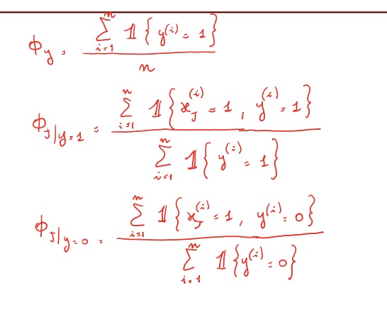
  Naive bayes is parametrized by:

  • ${\varphi }_{j|y=1}=P(x_j=1|y=1)$: the probability that the word $j$ is in the email, given that the email is spam;
  • ${\varphi }_{j|y=0}=P(x_j=1|y=0)$: the probability that the word $j$ is in the email, given that the email is not spam;
  • ${\varphi }_y=P(y=1)$: the probability that an email is a spam.

  We can apply MLE to obtain these parameter and make a prediciton.

  

• Multinomial event model

  This is a generalization of the naive bayes model. The formula to compute $P(x|y)$ is exactly the same, but the feature vector $x$ is different.

  Given a vocabolary of lenght $|V|$, we define $x_j$ as the index of the word in the vocabulary $V$.

  The feature vector $x$ is now an array of dimension ${\mathbb{R}}^{n_i}$ where $n_i$ is the lenght of the $i$-th email. The $j$-th element of the array is defined as $x_j$, meaning the index of the $j$-th word in the email in the vocabolary.

  $P(x_j|y)$ is now a multimodal probability instead of a bernoulli, so it’s a multiclass classifier.

  Also the $\varphi$ parameter is redefined as following:

  $$\begin{gathered} {\varphi }_{k|y=0}=P(x_j=k|y=0) \\ =\frac{{\sum }_{i=1}^{n}1\{y^{(i)}=0\}{\sum }_{i=1}^{n}1\{x_j^{(i)}=k\}+1}{{\sum }_{i=1}^{n}1\{y^{(i)}=0\}\cdot n_i+|V|} \end{gathered}$$

  Where $|V|$ (the size of the vocabulary) at the denominator and $1$ at the numerator are for laplace smoothing.

Performance evaluation

• Confusion matrix

  A confusion matrix is a structure where it’s possible to have a recap of the performance of the model.

  TP	FP
  FN	TN

• Accuracy, precision, recall, F1

  The following are metrics to evaluate the system performance, and allows to compare two or more systems.

  • Accuracy: $\frac{TN+TP}{N}$ describes how many true predictions the model made out of all the predictions. Describes the rate of correctness, and so also the rate of the wrong predictions.
  • Precision: $\frac{TP}{TP+FP}$ describes how good the model is at giving a positive result and actually being right about it. If I raise the threshold, the precision gets higher. This is useful in an emergency situation when I want to do something only if I am very sure about it. I can also apply this if I want to do some heavy calculations only on some occasions, and I want to be sure to do it correctly.
  • Recall (True Positive Rate or Sensitivity): $\frac{TP}{TP+FN}$ it describes how many true positives has the model found over all the positives. For example in the case of heart disease patients, a high recall is mandatory since with a low recall the model will not predict heart disease for a patient that actually has it.
  • Negative Recall (False Positive Rate or Specificity): $\frac{FP}{TN+FP}=1-\text{Specificity}$: it describes how many mistakes the model doing on the positives. For example in an emergency break on an autonomous car, I want this value to be very low otherwise it will be probable that an emergency brake will happen when it’s not necessary.
  • F1: $\left(\frac{2}{recal{l}^{-1}+precisio{n}^{-1}}\right)=2\frac{precision\cdot recall}{precision+recall}$. It’s a weighted average of precision and recall. F1 score is usually more useful than just accuracy, especially in uneven class distribution.

• ROC, AUC

  The ROC curve is a curve that allows to have an idea about the general performances of the model. It shows how the True positive rate (Recall) changes with respect to the False positive rate (Negative recall).

  An higher curve means higher performances. It’s possible to measure the “highness” of the curve by measuring the area under the curve (AUC) to have a single index of performances. A 0.5 area means that the model is just guessing.

Optimization methods

• Gradient descent

  Gradient descent is an iterative algorithm used to optimize a certain loss function.

  We start assigning a random value to the parameters, and then we update each of them at the same time according to this formula: ${\theta }_j:={\theta }_j-\alpha \frac{\partial }{\partial {\theta }_j}J({\theta }_0,{\theta }_1)$ , until convergence, or when the loss function value is very small or after a fixed number of iterations.

• Stochastic Gradient descent

  SGD is an optimized variant of the gradient descent in which not all the data points are used for the optimization at each iteration, but only one, or a small subset called mini-batch is used, in order for the algorithm to be usable on large datasets.

• Newton’s method

  It’s another iterative optimization algorithm that can be used as an alternative to gradient descent.

  Each time we update the parameter according to this formula: ${\theta }^{(t+1)}:={\theta }^{(t)}-\frac{{\ell }^{\prime }({\theta }^{(t)})}{{\ell }^{\prime \prime }({\theta }^{(t)})}$ where $\ell (\theta )$ is the log-likelihood of the loss function.

  The pro of this method is that there isn’t any hyperparameter, but the method requires an higher order of differentiability for the loss function.

  In case $\theta$ is a vector, we ca rewrite the formula to: ${\theta }^{(t+1)}:={\theta }^{(t)}-H^{-1}{\nabla }_{\theta }\ell$ where ${\nabla }_{\theta }\ell$ is the gradient of $\ell$ and $H$ is the hessian matrix which elements are defined as $H_{ij}=\frac{{\partial }^2\ell }{\partial {\theta }_i\partial {\theta }_j}$.

• Normal equation

  Normal equation is another optimization method that’s not iterative, and can be used to approximate the best parameters if the setup respects some costraints in sometimes a more efficient way.

  The idea is to minimize $J$ by explictly taking its derivative with respect to the ${\theta }_j$’s and setting them to zero.

  The final best parameters can be computed using this formula: $\theta =(X^{T}X{)}^{-1}{X}^T\overrightarrow{y}$ where

  • $X$ is the design matrix that contains the training examples and is in ${\mathbb{R}}^{n+1}$.
  • $\overrightarrow{y}\in {\mathbb{R}}^{n+1}$ is the vector containing the target values from the training set.

  We can see that in order for this to work, the design matrix $X$ has to be invertible, so it must be squared and its determinant cannot be zero. The matrix invertion operation has a computational complexity of $O(n^3)$.

  The matrix $X^{T}X$ is non-invertible if:

  • Reduntant feature exists (lineary dependent), such as a size in feet and a size in meters.
  • There are too many features with respect to the number of samples ($m\le n$), this can be solved by deleting some features (feature selection) or by using regularization.

• Maximum Likelihood Estimate

  Maximum likelihood estimate is the maximization of the likelihood done by minimizing the log-likelihood with techniques like gradient descent.

  The likelihood is defined as $L(\theta )=P(\overrightarrow{y}|X;\theta )={\prod }_{i=1}^{m}P(y^{(i)}|x^{(i)};\theta )$.

Generalization

• What is the exponential family of distributions?

  The exponential family is a set of distributions whose probability distribution can be described by a general equation:

  $$P(y|\eta )=b(y)\exp \left({\eta }^{T}T(y)-a(\eta )\right)$$

  Where:

  • $\eta$ is the natural parameter
  • $T(y)$ is the succifient statistic (most of the time $T(y)=y$)
  • $b(y)$ is the base measure (scalar)
  • $a(\eta )$ is the log-partition function
  • $y$ is the data (scalar)

  $\eta$ and $T(y)$ can be scalars or vectors, but their shape must match.

• Generalized Linear Models

  Generalized linear models are a generalization for all the models that follows the three following assumptions:

  1. $y|x;\theta \sim \text{ExpFamily}(\eta )$;
  2. Given $x$, we want to have $h_{\theta }(x)=E[T(y)|x]$;
  3. $\eta ={\theta }^{T}x$. If $\eta$ is a vector, then ${\eta }_i={\theta }_i^{T}x$, meaning that the parameter $\eta$ and the input are linearly related.

Neural Networks

• Neural Networks

  A neural network is a set of layers made up of neurons that are fully connected to the neurons of the next layer.

  The neurons are the data, the connection are the weights, that create linear combination between the neurons. There is also the bias, that is another parameter that adds up to the weight and the data in order to adjust the result and to allow the model to learn more complex patterns.

  The weights and bias are adjusted at every iteration with backpropagation.

• Backpropagation

  Just like gradient descent, we can be sure of the “direction” to adjust the weight in order for the model to perform better. The direction of a function is represented by its gradient, and backpropagation is an efficient way to compute the gradient for each neuron in the network.

  The idea is to start from the end of the network and recursively apply the chain rule to compute the gradients all the way to the inputs of the network, and then update the weights in the right direction.

  In each step of backpropagation, we compute the new gradient as the product between the upstream gradient and the local gradient. The upstream gradient is the gradient that comes from the backpropagation, the local gradient is the one that’s computed in the forward pass locally for each parameter.

  In case we’re dealing with vectors, matrices or tensors then the process is the same but we’re not computing regular derivatives anymore, but gradients or jacobians.

• Convolutional neural networks

  CNN are neural networks that use the kernel convolution operation in order to find the most important features, and then those features are passed to a fully connected neural network in order to make a prediction. They’re mostly used for image classification, since they learn both the most important features and the right classification, so there is no need to manually extract the features.

  There are three types of layers:

  • Convolutional layer: the image is convolved with a kernel that generates a smaller image but with the same depth (3 if RGB). Each kernel generates an image and all these images are stacked togheter forming an activation map, that’s smaller than the original but with an higher depth;
  • Activation Layer: the activation map is given in input to a certain activation function. This is needed in order to insert some non-linearity, otherwise the model coudn’t be able to learn more complex patterns.
  • Pooling Layer: pooling is an operation that takes a patch of an image and returns some ouput that’s smaller than the original image. It’s useful to reduce the image resolution. For examples it can return the average or the max of the values inside the patch. Differently then convolution, the patches don’t overlap.

• Activation functions

  Activation function is useful in order to insert some non-linearity inside of the model, in order for it to be able to learn more complex patterns. These are the most famous activation functions:

  • Sigmoid: $f(x)=\frac{1}{1+e^{-z}}\in [0,1]$
  • Tanh: $f(x)=\frac{2}{1+e^{-2x}}-1\in [-1,1]$
  • ReLU: $f(x) = \begin{cases} 0 && \text{for} \quad x\le0 \ x && \text{for} \quad x\ge0 \

  \end{cases} \in [0,x]$

  • Leaky ReLU: $f(x) = \begin{cases} \alpha x && \text{for} \quad x\le0 \ x && \text{for} \quad x\ge0 \

  \end{cases} \in [\alpha x, x]$

  • SoftPlus: $f(x)={\log }_e(1+e^x)\in [0,+\infty ]$

Regularization, bias and variance

• Regularization

  Regularization is needed in order to prevent the model to overfit. THis This is done by adding a certain factor $\lambda R(W)$ at the end of the loss function.

  There are many types of regularization, that make $R(W)$ change:

  • L2 regularization: $R(W)={\sum }_k{\sum }_l{W}_{k,l}^2$
  • L1 regularization: $R(W)={\sum }_k{\sum }_l|W_{k,l}|$
  • Elastic net (L1 + L2): $R(W)={\sum }_k{\sum }_l\beta W_{k,l}^2+|W_{k,l}|$

  $\lambda$ it’s an hyperparamter that models the regularization strength.

• Relationship between bias, variance, overfitting and underfitting

  • If the model underfits the data, is the situation of high bias and low variance (no matter how much data is given in input, the model will always perform bad);
  • If the model overifts the data, we’re in the situation of high variance and low bias (the prediction variates a lot depending on the input sample).

• High bias and how to fight it

  The bias is an error induced by approximating a real-life problem during the learning process, and so the model misses relvant relations between features and target, resulting in underfitting;

  It’s possible to fight it in the following ways:

  • Increase the number of features
  • Increase the grade of the polynomial in the hypothesis
  • Decreasing the regularization parameter

• High variance and how to fight it

  The variance is an error induced by the variability of the model’s prediction for the same input. A model with an high variance pays too much attention to the training data and doesn’t generalize well for testing data, resulting in overfitting.

  It’s possible to fight it in the following ways:

  • Use more data to train the model
  • Decreasing the model complexity by removing the number of fetatures or adding regularization and dropout

• Data view vs Parameter view

  Data view and parameter view are two differen types of methods to vieualize the prediciton made by the model:

  • Data view shows the prediction with respect to the dependent and independent variable ($x$ and $y$);
  • Parameter view shows the prediction with respect to the paramteres ($\theta$s).

  We call ${\theta }^{\ast }$ the optimal parameter, and $\hat{\theta }$ the predicted parameter.

  In the paramter view, the $x$ axis represents the variance and the $y$ axis represents the bias.

  The variance and bias can be visualized as:

  • Bias: how much far away are thre prediction from the center;
  • Variance: how much spread are the points between them.

• Consistent and unbiased algorithm

  • An algorithm is consistent if $\hat{\theta }\to {\theta }^{\ast }$ with data $m\to \infty$;
  • An algorithm is unbised if $E[\hat{\theta }]={\theta }^{\ast }\forall m$.

• Risk Empirical Risk and types of errors

  We can define the risk, or generalization error as $ϵ(h)=E_{(x,y)\sim D}[1\{h(x)\ne y\}]$, and is the error we get if we’d be able to train the model with infinite data.

  The empircal risk, defined as $\widehat{ϵ}(h{)}_s=\frac{1}{m}{\sum }_{i=1}^{m}1\{h(x)\ne y\}$, is the error we get training the model on $m$ samples.

  Let $g$ be the best hypothesis achievable with an infinite amount of data; $h^{\ast }$ the best hypothesis with achievable by all the possible models with a certain limited amount of data and $\hat{h}$ our estimate.

  From that we can define some types of errors:

  • $ϵ(g)$ is the Bayes error, or irreducible error. Is the minimum achievable error possible;
  • $ϵ(h^{\ast })-ϵ(g)$ is the approximation error, due to choice of parameters;
  • $ϵ(\hat{h})-ϵ(h^{\ast })$ is the estimation error, due to the limited amount of data.

  The generalization error $ϵ(h)$ can be computed as:

  $$ϵ(h)=\text{est error}+\text{approx error}+\text{irriducible error}$$

  We can also decompose $\text{est error}$ as $\text{est variance}+\text{est bias}$.

Other stuff

• Measuring correlation with the $r$ coefficient

  Two variables are correlated if they track each other. There could be positive correlation if their trend is similar (one goes up, the other goes up); or negative correlation if their trend is inverse (one goes up, the other goes down).

  Correlation is different from causation, which means that a value directly influences another.

  It’s possible to measure the level of correlation, while it’s almost impossible to find some causations.

  The level of correlation can be measured with the Pearson coefficient $r\in [-1,1]$. $-1$ meas highest negative correlation, $0$ means no correlation and $1$ highest positive correlation.

  It’s possible to square the coefficient to $r^2\in [0,1]$ in order to measure the correlation whitout caring about the sign.

• Gradient and magnitude

  Gradient is a vector that describes the direction and rate of the fastest increase or decrease of a function $f$ and it’s denoted as $\nabla f$.

  The vector is composed by the partial derivative with respect to all the possible function parameters:

  $$\nabla f(p)=\left[\begin{array}{c}\frac{\partial f}{\partial x_1}(p)\\ ⋮\\ \frac{\partial f}{\partial x_n}(p)\end{array}\right]$$

  The gradient magnitude is a scalar that measures the maximum rate of change. This is defined as $\Vert \nabla f\Vert =\sqrt{D_x^2+D_y^2}=\sqrt{{\sum }_{i=1}^n\nabla f^{(i{)}^2}}$.

  The direction of the gradient is given by $\theta =arctan(D_y,D_x)$.

• Gradient check

  Gradient check is a technique that allows to debug the backpropagation algorithm. The idea is to calculate the gradient in an analytical way, and compare the results with the backpropagation results. If they’re similar, then the process is correct, otherwise one of the two calculations must be wrong.

• Laplace smoothing

  Laplace smoothing is a technique in order to avoid a zero-probability for an event that it’s never been seen. The technique incluides adding $1$ for every positive observation and $1$ for every negative observation.

  This is done also to avoid overfitting and improving the general performance of the model.